


 Inglés (pdf)
 Articulo en XML
 Enviar articulo por email
 Permalink
1 Introduction
Quantitative based research in Education involving complete data analysis is highly improbable, particularly if the statistical unit of measurement is the human subject. Unanticipated events in data collection often cause missing data, attrition, and nonresponse. However, research papers in education often do not mention the occurrence of missing data ( COX et al., 2014 ; WELLS et al., 2015 ) despite best practice recommendations in reporting and handling missing data (PAMPAKA; HUTCHESON; WILLIAMS, 2016; SCHLOMER; BAUMAN; CARD, 2010) in quantitative based research. The American Psychological Association’s report ( WILKINSON; APA BOARD OF SCIENTIFIC AFFAIRS, 1999 ) on statistical methods in Psychology journals mentions that “The two popular methods for dealing with missing data that are found in basic statistics packages – listwise and pairwise deletion of missing values are among the worst methods available for practical applications” (p. 598). Since then the increasing use of alternative methods such as Maximum Likelihood (ML) estimation or Multiple Imputation (MI) ( RUBIN, 1987 ) has been reported by several authors ( COX et al., 2014 ; LAVANYA; REDDY; REDDY, 2019; PAMPAKA; HUTCHESON; WILLIAMS, 2016; PEUGH; ENDERS, 2004 ; SCHLOMER; BAUMAN; CARD, 2010). An extensive review of practices dealing with missing data in the educational and psychological research was conducted by Peugh and Enders (2004) , who divided the missing data methods into two categories: the “traditional” and the “modern” methods, which include ML and MI. The articles reviewed were published in 16 educational and applied psychological journals in 1999 and 2003. According to authors, in 1999, 33.75% of the papers explicitly reported the problem of missing data and in 2003 such percentage more than doubled (74.24%). In addition, in 1999 none of the papers in the review adopted ML or MI for missing data handling, and they reported six papers in 2003. In fact, the field of education and other related disciplines have been strongly conditioned either by the availability of data or by their quality ( FOLEY; GOLDSTEIN, 2012 ). On the American Statistical Association’s statement to inform the use of Value Added Models (VAMs) “for educational assessment […] where states and local governments use them to make high-stakes decisions regarding teacher performance appraisals and compensation” ( MORGANSTEIN; WASSERSTEIN, 2014 , p. 108) the authors state that the models “can help evaluate teaching programs […]”, and conclude that their use must regard for data and statistical model assumptions and limitations. We face “The challenge with VAMs is to include all the important factors that might contribute to the observed differences in test scores. Many potential explanatory variables are not available for inclusion or have many missing values […]” ( MORGANSTEIN; WASSERSTEIN, 2014 , p. 109). Therefore, no matter how large the volume of data is, how high the velocity is, or how many formats are available, the problem of missingness also strongly affects big identifiable data, implying that their use for policy and practice in Education imposes the adoption of proper strategies of missing data handling. Most of the quantitative based literature in educational research include the following variables as attributes of interest: student’s achievement, national exams scores, grade repetition, and individual sociodemographic characteristics such as gender and socioeconomic status (SES). In order to monitor and promote the equity of an education system, one of the key variables is the student’s SES (e.g. Author, 2015). The variable commonly used as proxy is mother’s education, which very often reaches more than 20% of missing values. The Missing Completely At Random (MCAR) assumption ( LITTLE, 1988 ) when data modelling implies that the respective students are excluded from the analyses. Since the most needy students in public education are the most likely not to answer such key variables, any educational performance indicators based on naïve assumptions may fail to properly quantify the school effects and, thus, fail to promote the reduction of educational and social inequalities.
COX et al. (2014) reviewed the topic in the field of higher education scientific literature and conclude that “multiple imputation has emerged as the preferred option among statisticians and sociologists, who have been employing advanced methods for more than a decade” (p. 387), and they also refer multiple imputation procedures available in several commercial software packages. Thus, authors argue that “multiple imputation should be the new default option for quantitative research in higher education” (p. 387).
Two main contributions arise from this paper. Firstly, we explain in detail and illustrate with real-world data how the researcher should test if the missing data are MCAR. Second, we show the impact of assuming MCAR or running MI on the linear relationship between student’s performance and student’s socioeconomic status by comparing descriptive statistics and linear regression coefficient estimates. We will apply a routine for LITTLE (1988) ’s hypothesis test and the R package for multiple imputation procedures to Prova Brasil data collected in 2017 in the Northeast and South regions.
The remainder of this paper consists of three parts. Section two proceeds to the review of the scientific literature published in Brazilian and Portuguese journals registered in the SciELO platform. Section three presents data and methods, comprising the explanation of statistical packages in R to check the pattern of missingness and to conduct multiple imputation. Finally, the discussion and conclusion as section four. To our knowledge this is the first paper to present MI applied to big identifiable data of Prova Brasil and to evaluate the impact of naïve assumption as MCAR.
2 Missing data in the Brazilian educational research
The heart of this section is a review of the relevant quantitative research in education and educational research registered in the SciELO platform. The primary interest of this study is to identify the methods in use for missing data treatment in quantitative research that used Prova Brasil data. This paper focuses on studies published from 2016 to 2018. The main objective of the review process was to identify as many relevant and high-quality articles as possible. Thus, our strategy was to search a wide variety of papers and then systematically eliminate those that did not meet the criteria for content or relevance. The first step of the review was to conduct a search for peer-reviewed papers published from 2016 to 2018 using the SciELO search engine covering the education and educational research literatures. The search was conducted during May 2019. We searched for papers that listed “Prova Brazil” or “Prova Brasil” as a keyword or included the term in the abstract. The filter was (prova brasil) OR (prova brazil) AND year_cluster:(“2016” OR “2018” OR “2017”) AND work_subject_categories:(“education & educational research”) AND type:(“research-article”). We found 15 papers. Then, the content search was limited to papers that included “missing” data, dado “ faltante ” ou dado “ omisso ” (SOCIEDADE PORTUGUESA DE ESTATÍSTICA; ASSOCIAÇÃO BRASILEIRA DE ESTATÍSTICA, 2011) in the methodology section. We also looked up the tables and descriptive statistics in order to find out how missing data were treated. Four papers are narratives on evaluation or assessment and one presents a historical perspective. Amongst the remaining papers, four mentioned the existence of missing data ( BARTHOLO; COSTA, 2016 ; FONSECA; NAMEN, 2016 ; OLIVEIRA; CARVALHO, 2018 ; PONTES; SOARES, 2017) , but none of them explicitly mentioned any assumption or method to deal with missing data. Facing the short number of papers that recently have used the large and complex data Prova Brasil , we decided to extend the search for articles going back to the beginning of the century, thus the time period was 2000–2018 and enlarging the search for the periodic Estudos de Avaliação Educacional , which is not registered in Scielo platform. It is well-reputed by educational researchers. Thus, we looked for the keywords or expressions (and variations) in Portuguese or in the language of the article: “missing”/“ omisso ”/“ faltante ”, “missing data”/“ dados omissos ”/“ dados faltantes ”, “incomplete data”/“ dados incompletos ” and “no response”/“ sem resposta ”. The content analysis was focused on the methodology and results sections. We found 60 papers, which 38% (23) explicitly mention missing data, and 30% (18) apply a method to deal with the problem. The vast majority, that is 16 out of 18 papers, used a traditional method of imputation, meaning that, in general, ML and MI have been seldom used by educational researchers.
Vinha and Laros (2018) conducted a simulation study with the Brazilian education assessment data including 7,000 cases and eight variables which comprise four as auxiliary variables, in order to compare the performance of methods for missing treatment (mean imputation, listwise deletion, ML and MI). They confirmed that the mean imputation showed the worst performance. Their analyses were conducted using a commercial software.
Ferrão and Prata (2019) used R open source software to test the pattern of missingness in simulated datasets generated from Prova Brasil 2017. They were generated to include MCAR or non-ignorable missing data ( LITTLE, 1988 ). In the first situation, ML or MI procedures can be avoided without detriment of results. The Prova Brasil 2017 was used as big identifiable data ( SHLOMO; GOLDSTEIN, 2015 ) in educational research. They run MI with R and concluded that for datasets of about 20,000 cases and three variables, one auxiliary variable, the execution time does not depend on the missing percentage, varying between 5% and 20%. Increasing the number of cases (more than half a million) and the number of variables (10) with missing (8), the MI execution time was 116.4 minutes using a computer 8 GB RAM and 30.8 minutes with a computer 16 GB RAM. In addition, they mentioned that the routine run with four chains in parallel, with a limit of 35 iterations, but some variables had not converged. In fact, the use of big data for research purposes, may be an opportunity or a threat ( DIGGLE, 2015 ), if the big data do not cover the entire target population or there is a selective mechanism that produces missing data that are not MCAR, the research itself may be compromised.
3 Methodology
As an example of educational research where identifiable big data ( SHLOMO; GOLDSTEIN, 2015 ) do not cover the entire target population and, thus, the missing subjects may not be completely at random, we used the Prova Brasil 2017 data.
3.1 Prova Brasil 2017 data
The education data used in this study is the Avaliação Nacional do Rendimento Escolar (INEP - INSTITUTO NACIONAL DE ESTUDOS E PESQUISAS EDUCACIONAIS ANÍSIO TEIXEIRA, 2018), well known as Prova Brasil . The Prova Brasil was created in 2005 under the scope of the Basic Education Assessment System (Saeb) with the aim of assessing students learning at Brazilian public schools. It is a quasi-census type applied to students at the 5th and 9th grades of primary education in schools with 20 or more students enrolled in these grades. It covers all Brazilian territory and is carried out every two years by the Instituto Nacional de Estudos e Pesquisas Educacionais Anísio Teixeira (Inep), which is responsible for developing and applying educational assessments, and also the census of education. The Prova Brasil comprises standardized tests on Portuguese Language (reading) and Mathematics, as well as questionnaires targeting students, teachers, principals and schools. Saeb’s proficiency scales range from 0 to 500 with mean 250 and standard deviation 50 to 9th grade students ( KLEIN, 2003 ). Inep defined the eligible population for Prova Brasil based on the consolidated data of the Basic Education School Census of 2017.
We excluded from our analyses the federal schools, which represent 0.04% of public schools and are very different from common public schools in terms of student profile, infrastructure and organization. After this exclusion, the finite population is, then, a large identifiable sample of size N = 2,594 million students of its superpopulation of the 5th grade. The performance scores in Math and Reading are available for 2,170 (84%) million students and the socioeconomic status for 2,132 (82%) million students.
Table 1 summarizes the data patterns with respect to the missing data problem. Note that the main occurrence of missing data is due to the eligible students who did not attend school on the day of Prova Brasil (16.23%) administration. Other students attended the school that day, but did not take the test, neither answered the questionnaire (0.09%); others just did the test (0.65%), and a few of them were not present on the test day but filled in the questionnaire (0.04%). In several educational research studies, missing data are due to item nonresponse, i.e., participants in a survey or test who do not give responses for every item administered [item missing]. In addition, the expected participants in the survey or test do not appear [subject missing]. In the Brazilian data, comparing to the target population, there are at least 17% of subject missing and 83% with valid data but item missing. This study is focused on MI applied to item missing.
Table 1 Distribution of missing and valid data of 5th grade students eligible for the Prova Brasil in state and municipal schools – 2017
| N | Percentage | |
|---|---|---|
| Student did not attend school on t day | 421,084 | 16.23 |
| Student attended but did not take the test, nor filled in the questionnaire | 2,239 | 0.09 |
| Student took the test, but not filled in the questionnaire | 16,866 | 0.65 |
| Student did not take the test, but filled in the questionnaire | 1,015 | 0.04 |
| Student took the test and questionnaire (fully or partially) | 2,153,131 | 82.99 |
| Total | 2,594,335 | 100.0 |
Source: own calculation (2019)
For the purpose of this paper, we chose to analyze data related to every Federation Unit (FU) in the Northeast and South regions of Brazil, because these regions are very different in many socio-educational dimensions. In addition, we decided to conduct the missing data analysis extending the simulation work described by Ferrão and Prata (2019) . Thus, the data analysis comprises three variables: student’s performance in reading (PR), student’s socioeconomic status (SES) and student’s trajectory without grade repetition (AP - which stands for “always promoted”). The student’s situation on promotion (always promoted vs. grade repetition) is considered a complete data variable and it is used as auxiliary variable for the MI purposes. In fact, it is possible to get such a complete data variable from the Brazilian school census and administrative data merging.
The student’ SES was calculated by applying the graded response model ( SAMEJIMA, 1997 ) to items of the student’s questionnaire, such as items regarding comfort goods (TV, automobile, computer, refrigerator, etc.), hiring of housekeeper and parents’ education (ALVES; SOARES; XAVIER, 2014).
Table 2 shows for each FU of the studied regions the number of observations and the percentage of missing values in SES and PR variables. As can be observed, the percentage of missing values in the northeast region is much higher than in the south. In the northeast the percentage of missing values for both variables are between 15 and 24.0% with the exception of the PR variable in the FU 23 (Ceará) that has just 8.6% of missing values. In the south, the missing percentage of both variables is between 3 and 7.0%. While in the northeast the percentage of missing values for SES variable is higher than for PR variable, with just one exception (FU = 24), in the south the opposite occurs. Here, the missing percentage for PR is always higher than the missing percentage in SES. It should be noted that if a student answered just to 3 or less items of a test, his performance was not calculated.
Table 2 Number of observations and the percentage of missing values for each studied FU
| Northeast | SES (Missing percentage) | PR (Missing percentage) | Number of observations |
|---|---|---|---|
| FU = 21, Maranhão | 21.9 | 20.9 | 62,249 |
| FU = 22, Piauí | 20.6 | 15.7 | 29,700 |
| FU = 23, Ceará | 20.4 | 8.6 | 86,628 |
| FU = 24, Rio Grande do Norte | 15.7 | 18.3 | 24,690 |
| FU = 25, Paraíba | 18.7 | 16.4 | 25,795 |
| FU = 26, Pernambuco | 18.8 | 15.8 | 72,738 |
| FU = 27, Alagoas | 23.6 | 17.6 | 32,143 |
| FU = 28, Sergipe | 20.6 | 19.6 | 19,422 |
| FU = 29, Bahia | 16.4 | 15.8 | 104,778 |
| South | |||
| FU = 41, Paraná | 3.9 | 4.9 | 104,916 |
| FU = 42, Santa Catarina | 2.9 | 5.5 | 65,985 |
| FU = 43, Rio Grande do Sul | 3.1 | 7.1 | 70,368 |
Source: own calculation (2019)
Descriptive statistics for SES variable of the studied data are presented in Table 3 . Considering that valid values of the SES variable are between 0 and 10, it can be observed that the mean and the median of SES variable have values below 50% of the full scale in the entire northeast region. On the contrary, in the entire south region the mean and median values for SES variable are greater than 5.5, i.e., in the second half of the scale.
Table 3 Descriptive statistics of SES variable with missing values by FU
| FU | Minimum | 1st Quartile | Median | Mean | 3rd Quartile | Maximum |
|---|---|---|---|---|---|---|
| 21 | 0.200 | 4.200 | 4.600 | 4.726 | 5.300 | 9.700 |
| 22 | 0.500 | 4.100 | 4.600 | 4.715 | 5.300 | 9.600 |
| 23 | 0.000 | 4.200 | 4.700 | 4.729 | 5.300 | 9.700 |
| 24 | 0.300 | 4.300 | 4.800 | 4.924 | 5.500 | 9.700 |
| 25 | 0.000 | 4.200 | 4.700 | 4.805 | 5.400 | 9.700 |
| 26 | 0.300 | 4.200 | 4.700 | 4.779 | 5.300 | 9.700 |
| 27 | 0.100 | 4.000 | 4.600 | 4.606 | 5.200 | 9.700 |
| 28 | 0.500 | 4.200 | 4.700 | 4.727 | 5.300 | 9.700 |
| 29 | 0.000 | 4.300 | 4.800 | 4.885 | 5.500 | 9.700 |
| 41 | 0.400 | 4.900 | 5.500 | 5.639 | 6.300 | 9.700 |
| 42 | 1.300 | 5.000 | 5.700 | 5.734 | 6.400 | 9.700 |
| 43 | 0.100 | 5.000 | 5.600 | 5.727 | 6.400 | 9.700 |
Source: own calculation (2019)
Finally, descriptive statistics of PR variable are presented in Table 4 . The PR variable is standardised, and as can be observed, its mean and median values are negative in the northeast region, with the exception of Ceará. In the south region, the opposite occurs, mean and median are always positive.
Table 4 Descriptive statistics of PR variable with missing values by FU
| FU | Minimum | 1st Quartile | Median | Mean | 3rd Quartile | Maximum |
|---|---|---|---|---|---|---|
| 21 | -2.400 | -0.800 | -0.300 | -0.289 | 0.300 | 2.500 |
| 22 | -2.400 | -0.600 | -0.100 | -0.300 | 0.600 | 2.500 |
| 23 | -2.400 | -0.300 | 0.400 | 0.370 | 1.000 | 2.500 |
| 24 | -2.400 | -0.700 | -0.200 | -0.147 | 0.400 | 2.500 |
| 25 | -2.400 | -0.700 | -0.100 | -0.087 | 0.500 | 2.500 |
| 26 | -2.400 | -0.600 | -0.100 | -0.049 | 0.500 | 2.500 |
| 27 | -2.400 | -0.700 | -0.100 | -0.082 | 0.500 | 2.500 |
| 28 | -2.400 | -0.800 | -0.300 | -0.271 | 0.300 | 2.500 |
| 29 | -2.400 | -0.600 | -0.100 | -0.080 | 0.500 | 2.500 |
| 41 | -2.300 | -0.100 | 0.400 | 0.439 | 1.000 | 2.500 |
| 42 | -2.400 | -0.100 | 0.400 | 0.454 | 1.000 | 2.500 |
| 43 | -2.400 | -0.300 | 0.300 | 0.305 | 0.900 | 2.500 |
Source: own calculation (2019)
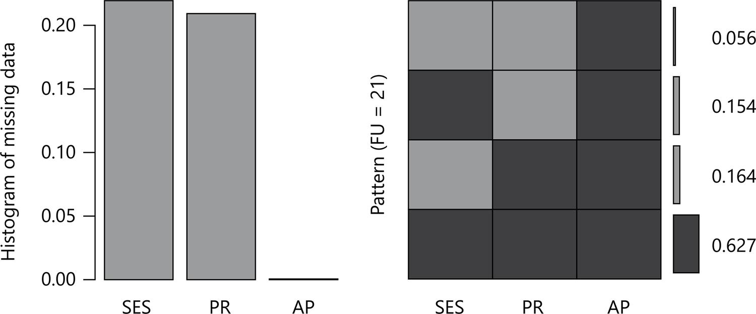
The datasets have four missing patterns, which are illustrated in Figure 1 for FU 21 (in the left hand side) and FU 43 (in the right hand side). For each FU the empirical distribution and the pattern of missing values are presented. As can be observed in both cases, the missing pattern with a small number of observations is the one with two missing variables.
3.2 MCAR test
As described in the literature ( FERRÃO; PRATA, 2019 ; IBRAHIM et al., 2005 ; VINHA; LAROS, 2018a), a common concern of every social and educational data scientist when he starts the analysis of multivariate data with missing values is checking if missing data are MCAR. We applied the test of hypothesis proposed by ( LITTLE, 1988 ) and implemented in R.
For that purpose the function LittleMCAR from the BaylorEdPsych package was used. BaylorEdPsych is an R package for Baylor University Educational Psychology Quantitative Courses ( BEAUJEAN, 2015 ) that uses Little’s test to assess for MCAR for multivariate data with missing values. It receives as argument a data frame or a data matrix with no more than 50 variables. Running the LittleMCAR function on every studied dataset we got a p-value of 0.0, conducting to the rejection of the null hypothesis, and concluding that the missingness pattern is not MCAR. The respective chi-square values, computed with 5 degrees of freedom, are presented in Table A1 in the annex.
3.3 Multiple Imputation
Multiple Imputation is a technique that involves creating m>1 multiple simulated values to replace each missing value. Then, each plausible version of the m complete datasets is analyzed as if it were a real complete dataset, by applying any standard statistical method. For a matter of inference, some authors (e.g. Ibrahim et al.) suggest obtaining one result by averaging over the m filled-in datasets; others (e.g. Peugh; Enders, 2004) suggest obtaining “A single estimand […] for any parameter by taking the arithmetic average of that parameter across the m analyses” (p. 550).
Concerning the UFs chosen, we used the package mi (Missing Data Imputation and Model Checking) to perform multiple imputation. That package imputes missing values in an approximate Bayesian framework ( GELMAN et al., 2015 ) generating multiple chains of values with a pre-defined number of iterations.
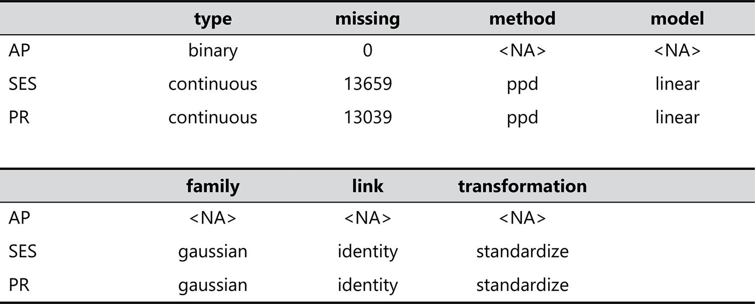
Before the imputation procedure, the dataset must be converted into a missing_data.frame object. That object will include metadata describing the variables with missing values and how they relate to each other. Variables are characterized with a type and a family. Figure 2 shows, as an example, the classification assigned to the dataset from the FU 21. As can be seen, the imputation method that will be used is the posterior predictive distribution (ppd). The classification and imputation method can be modified with a change function, according to the knowledge the user has about the data.
After analyzing the missing_data.frame, the imputation process can be done, calling the mi function. We choose to run 5 chains (m = 5) performing 35 iterations each. At the end, convergence between chains must be checked using the Rhats function. If the chains have not converged, the iterative process should continue using a second mi function that receives the result of the first call and the number of additional iterations. Finally, the imputation data can be collected using the mi2stata function. It allows exporting the data of all the chains to Stata (.dta) or comma separated (.csv) format.
Next section presents descriptive results (Tables 5 and 6), the m = 5 estimates for each set of regression model parameters in Table A2 in the annex, and in Table 7 the average of such estimates and standard errors, following Peugh and Enders (2004 , p. 550–551). The MI standard error (SE) estimated for each regression coefficient is given by equation (1), denoted by √T, and combines the within-imputation variance and the between-imputation variance,
Table A2 MI Estimates with m = 5
| UF-dataset | Const | SES coeff | AP coeff | UF-dataset | Const | SES coeff | AP coeff |
|---|---|---|---|---|---|---|---|
| 21-ori | -1.260 | 0.115 | 0.597 | 27-ori | -0.960 | 0.091 | 0.651 |
| 21-c-1 | -1.277 | 0.114 | 0.574 | 27-c-1 | -0.974 | 0.088 | 0.642 |
| 21-c-2 | -1.280 | 0.114 | 0.580 | 27-c-2 | -1.019 | 0.096 | 0.648 |
| 21-c-3 | -1.307 | 0.119 | 0.583 | 27-c-3 | -0.989 | 0.091 | 0.645 |
| 21-c-4 | -1.275 | 0.112 | 0.581 | 27-c-4 | -0.999 | 0.094 | 0.639 |
| 21-c-5 | -1.293 | 0.116 | 0.580 | 27-c-5 | -1.011 | 0.096 | 0.640 |
| 22-ori | -0.886 | 0.098 | 0.601 | 28-ori | -0.906 | 0.067 | 0.512 |
| 22-c-1 | -0.906 | 0.099 | 0.583 | 28-c-1 | -0.940 | 0.068 | 0.520 |
| 22-c-2 | -0.924 | 0.103 | 0.580 | 28-c-2 | -0.930 | 0.068 | 0.502 |
| 22-c-3 | -0.899 | 0.097 | 0.586 | 28-c-3 | -0.926 | 0.068 | 0.498 |
| 22-c-4 | -0.903 | 0.098 | 0.586 | 28-c-4 | -0.895 | 0.059 | 0.512 |
| 22-c-5 | -0.900 | 0.095 | 0.600 | 28-c-5 | -0.939 | 0.069 | 0.508 |
| 23-ori | -0.414 | 0.063 | 0.619 | 29-ori | -0.807 | 0.074 | 0.549 |
| 23-c-1 | -0.429 | 0.063 | 0.607 | 29-c-1 | -0.835 | 0.076 | 0.536 |
| 23-c-2 | -0.425 | 0.062 | 0.607 | 29-c-2 | -0.819 | 0.072 | 0.543 |
| 23-c-3 | -0.433 | 0.064 | 0.606 | 29-c-3 | -0.830 | 0.075 | 0.536 |
| 23-c-4 | -0.426 | 0.062 | 0.609 | 29-c-4 | -0.826 | 0.075 | 0.533 |
| 23-c-5 | -0.427 | 0.064 | 0.604 | 29-c-5 | -0.826 | 0.075 | 0.534 |
| 24-ori | -1.128 | 0.099 | 0.695 | 41-ori | -0.520 | 0.088 | 0.567 |
| 24-c-1 | -1.153 | 0.102 | 0.677 | 41-c-1 | -0.536 | 0.090 | 0.563 |
| 24-c-2 | -1.147 | 0.099 | 0.684 | 41-c-2 | -0.528 | 0.089 | 0.562 |
| 24-c-3 | -1.119 | 0.095 | 0.677 | 41-c-3 | -0.531 | 0.089 | 0.566 |
| 24-c-4 | -1.169 | 0.104 | 0.677 | 41-c-4 | -0.532 | 0.089 | 0.562 |
| 24-c-5 | -1.146 | 0.098 | 0.689 | 41-c-5 | -0.528 | 0.088 | 0.565 |
| 25-ori | -0.873 | 0.081 | 0.578 | 42-ori | -0.803 | 0.121 | 0.660 |
| 25-c-1 | -0.892 | 0.083 | 0.559 | 42-c-1 | -0.817 | 0.121 | 0.663 |
| 25-c-2 | -0.862 | 0.078 | 0.549 | 42-c-2 | -0.806 | 0.121 | 0.652 |
| 25-c-3 | -0.879 | 0.079 | 0.559 | 42-c-3 | -0.819 | 0.122 | 0.663 |
| 25-c-4 | -0.876 | 0.080 | 0.554 | 42-c-4 | -0.820 | 0.122 | 0.662 |
| 25-c-5 | -0.863 | 0.079 | 0.549 | 42-c-5 | -0.799 | 0.120 | 0.654 |
| 26-ori | -0.736 | 0.059 | 0.577 | 43-ori | -0.859 | 0.125 | 0.562 |
| 26-c-1 | -0.749 | 0.059 | 0.572 | 43-c-1 | -0.878 | 0.127 | 0.561 |
| 26-c-2 | -0.752 | 0.057 | 0.577 | 43-c-2 | -0.866 | 0.125 | 0.560 |
| 26-c-3 | -0.772 | 0.061 | 0.576 | 43-c-3 | -0.880 | 0.128 | 0.561 |
| 26-c-4 | -0.754 | 0.058 | 0.577 | 43-c-4 | -0.870 | 0.126 | 0.564 |
| 26-c-5 | -0.766 | 0.061 | 0.573 | 43-c-5 | -0.872 | 0.126 | 0.563 |
Source: own calculation (2019)
Table 7 MCAR and MI estimates in the linear regression model
| MCAR | MI | ||||||||
|---|---|---|---|---|---|---|---|---|---|
| FU | R2 | Const | SES coeff | AP coeff | R2 | Const | SES coeff | AP coeff | |
| 21 | Parameter estimates | 0.10 | -1.260 | 0.115 | 0.597 | 0.11 | -1.286 | 0.115 | 0.580 |
| Standard error | 0.021 | 0.004 | 0.010 | 0.025 | 0.006 | 0.013 | |||
| 22 | Parameter estimates | 0.11 | -0.886 | 0.098 | 0.601 | 0.12 | -0.906 | 0.098 | 0.587 |
| Standard error | 0.029 | 0.006 | 0.013 | 0.025 | 0.006 | 0.013 | |||
| 23 | Parameter estimates | 0.07 | -0.414 | 0.063 | 0.619 | 0.07 | -0.428 | 0.063 | 0.607 |
| Standard error | 0.018 | 0.004 | 0.009 | 0.016 | 0.003 | 0.008 | |||
| 24 | Parameter estimates | 0.012 | -1.128 | 0.099 | 0.695 | 0.14 | -1.147 | 0.100 | 0.681 |
| Standard error | 0.034 | 0.007 | 0.015 | 0.033 | 0.006 | 0.013 | |||
| 25 | Parameter estimates | 0.09 | -0.873 | 0.081 | 0.578 | 0.09 | -0.874 | 0.080 | 0.554 |
| Standard error | 0.032 | 0.006 | 0.014 | 0.028 | 0.005 | 0.012 | |||
| 26 | Parameter estimates | 0.08 | -0.736 | 0.059 | 0.577 | 0.09 | -0.759 | 0.059 | 0.575 |
| Standard error | 0.020 | 0.004 | 0.009 | 0.019 | 0.004 | 0.007 | |||
| 27 | Parameter estimates | 0.10 | -0.960 | 0.091 | 0.651 | 0.11 | -0.998 | 0.093 | 0.643 |
| Standard error | 0.030 | 0.006 | 0.015 | 0.029 | 0.006 | 0.012 | |||
| 28 | Parameter estimates | 0.09 | -0.906 | 0.067 | 0.512 | 0.10 | -0.926 | 0.066 | 0.508 |
| Standard error | 0.036 | 0.007 | 0.015 | 0.033 | 0.007 | 0.015 | |||
| 29 | Parameter estimates | 0.09 | -0.807 | 0.074 | 0.549 | 0.09 | -0.827 | 0.074 | 0.536 |
| Standard error | 0.016 | 0.003 | 0.007 | 0.014 | 0.003 | 0.007 | |||
| 41 | Parameter estimates | 0.08 | -0.520 | 0.088 | 0.567 | 0.09 | -0.531 | 0.089 | 0.564 |
| Standard error | 0.015 | 0.003 | 0.007 | 0.015 | 0.003 | 0.007 | |||
| 42 | Parameter estimates | 0.10 | -0.803 | 0.121 | 0.660 | 0.11 | -0.812 | 0.121 | 0.659 |
| Standard error | 0.021 | 0.003 | 0.010 | 0.022 | 0.003 | 0.010 | |||
| 43 | Parameter estimates | 0.10 | -0.859 | 0.125 | 0.562 | 0.11 | -0.873 | 0.126 | 0.562 |
| Standard error | 0.019 | 0.003 | 0.008 | 0.019 | 0.003 | 0.007 | |||
Source: own calculation (2019)
where U̅ is the within-imputation variance and B is the between-imputation variance. Table A3 in the annex contains the standard error estimates for each chain.
Table A3 MI SE Estimates with m = 5
| UF-dataset | Const se_coeff | SES se_coeff | AP se_coeff | UF-dataset | Const se_coeff | SES se_coeff | AP se_coeff |
|---|---|---|---|---|---|---|---|
| 21-ori | 0.016 | 0.003 | 0.007 | 27-ori | 0.030 | 0.006 | 0.015 |
| 21-c-1 | 0.029 | 0.006 | 0.013 | 27-c-1 | 0.023 | 0.005 | 0.011 |
| 21-c-2 | 0.023 | 0.005 | 0.010 | 27-c-2 | 0.023 | 0.005 | 0.011 |
| 21-c-3 | 0.023 | 0.005 | 0.010 | 27-c-3 | 0.023 | 0.005 | 0.011 |
| 21-c-4 | 0.023 | 0.005 | 0.010 | 27-c-4 | 0.023 | 0.005 | 0.011 |
| 21-c-5 | 0.023 | 0.005 | 0.010 | 27-c-5 | 0.023 | 0.005 | 0.011 |
| 22-ori | 0.023 | 0.005 | 0.010 | 28-ori | 0.036 | 0.007 | 0.015 |
| 22-c-1 | 0.018 | 0.004 | 0.009 | 28-c-1 | 0.028 | 0.006 | 0.012 |
| 22-c-2 | 0.015 | 0.003 | 0.008 | 28-c-2 | 0.028 | 0.006 | 0.012 |
| 22-c-3 | 0.015 | 0.003 | 0.008 | 28-c-3 | 0.028 | 0.006 | 0.012 |
| 22-c-4 | 0.016 | 0.003 | 0.008 | 28-c-4 | 0.028 | 0.006 | 0.012 |
| 22-c-5 | 0.016 | 0.003 | 0.008 | 28-c-5 | 0.028 | 0.006 | 0.012 |
| 23-ori | 0.015 | 0.003 | 0.008 | 29-ori | 0.016 | 0.003 | 0.007 |
| 23-c-1 | 0.034 | 0.007 | 0.015 | 29-c-1 | 0.013 | 0.003 | 0.005 |
| 23-c-2 | 0.027 | 0.005 | 0.012 | 29-c-2 | 0.013 | 0.003 | 0.005 |
| 23-c-3 | 0.028 | 0.005 | 0.012 | 29-c-3 | 0.013 | 0.003 | 0.005 |
| 23-c-4 | 0.027 | 0.005 | 0.012 | 29-c-4 | 0.013 | 0.003 | 0.005 |
| 23-c-5 | 0.028 | 0.005 | 0.012 | 29-c-5 | 0.013 | 0.003 | 0.005 |
| 24-ori | 0.027 | 0.005 | 0.012 | 41-ori | 0.015 | 0.003 | 0.007 |
| 24-c-1 | 0.032 | 0.006 | 0.014 | 41-c-1 | 0.015 | 0.002 | 0.006 |
| 24-c-2 | 0.025 | 0.005 | 0.011 | 41-c-2 | 0.015 | 0.002 | 0.006 |
| 24-c-3 | 0.025 | 0.005 | 0.011 | 41-c-3 | 0.015 | 0.002 | 0.006 |
| 24-c-4 | 0.025 | 0.005 | 0.011 | 41-c-4 | 0.015 | 0.002 | 0.006 |
| 24-c-5 | 0.025 | 0.005 | 0.011 | 41-c-5 | 0.015 | 0.002 | 0.006 |
| 25-ori | 0.025 | 0.005 | 0.011 | 42-ori | 0.021 | 0.003 | 0.010 |
| 25-c-1 | 0.020 | 0.004 | 0.009 | 42-c-1 | 0.020 | 0.003 | 0.009 |
| 25-c-2 | 0.016 | 0.003 | 0.007 | 42-c-2 | 0.020 | 0.003 | 0.009 |
| 25-c-3 | 0.016 | 0.003 | 0.007 | 42-c-3 | 0.020 | 0.003 | 0.009 |
| 25-c-4 | 0.016 | 0.003 | 0.007 | 42-c-4 | 0.020 | 0.003 | 0.009 |
| 25-c-5 | 0.016 | 0.003 | 0.007 | 42-c-5 | 0.020 | 0.003 | 0.009 |
| 26-ori | 0.016 | 0.003 | 0.007 | 43-ori | 0.019 | 0.003 | 0.008 |
| 26-c-1 | 0.016 | 0.003 | 0.007 | 43-c-1 | 0.018 | 0.003 | 0.007 |
| 26-c-2 | 0.029 | 0.006 | 0.013 | 43-c-2 | 0.018 | 0.003 | 0.007 |
| 26-c-3 | 0.023 | 0.005 | 0.010 | 43-c-3 | 0.018 | 0.003 | 0.007 |
| 26-c-4 | 0.023 | 0.005 | 0.010 | 43-c-4 | 0.018 | 0.003 | 0.007 |
| 26-c-5 | 0.023 |
Source: own calculation (2019)
4 Results
Descriptive statistics of the imputed values, for each data set, are shown in tables 5 and 6. As example, we chose the results of chain 1. Table 5 presents the statistics by FU for the SES variable and table 6 for the PR variable.
Table 5 Descriptive statistics of SES variable for imputed data by FU
| FU | Minimum | 1st Quartile | Median | Mean | 3rd Quartile | Maximum |
|---|---|---|---|---|---|---|
| 21 | 0.100 | 4.070 | 4.600 | 4.678 | 5.300 | 9.700 |
| 22 | 0.500 | 4.100 | 4.660 | 4.708 | 5.300 | 9.600 |
| 23 | 0.000 | 4.100 | 4.700 | 4.724 | 5.300 | 9.700 |
| 24 | 0.300 | 4.300 | 4.800 | 4.916 | 5.500 | 9.700 |
| 25 | 0.000 | 4.200 | 4.700 | 4.794 | 5.400 | 9.700 |
| 26 | 0.300 | 4.200 | 4.700 | 4.774 | 5.400 | 9.700 |
| 27 | 0.100 | 3.910 | 4.600 | 4.595 | 5.210 | 9.700 |
| 28 | 0.500 | 4.100 | 4.700 | 4.727 | 5.300 | 9.700 |
| 29 | 0.000 | 4.300 | 4.800 | 4.879 | 5.500 | 9.700 |
| 41 | 0.400 | 4.900 | 5.560 | 5.636 | 6.300 | 9.700 |
| 42 | 1.300 | 5.000 | 5.700 | 5.732 | 6.400 | 9.700 |
| 43 | 0.100 | 5.000 | 5.600 | 5.724 | 6.400 | 9.700 |
Source: own calculation (2019)
Table 6 Descriptive statistics of PR variable for imputed data by FU
| FU | Minimum | 1st Quartile | Median | Mean | 3rd Quartile | Maximum |
|---|---|---|---|---|---|---|
| 21 | -3.920 | -0.900 | -0.360 | -0.315 | 0.240 | 2.500 |
| 22 | -3.530 | -0.700 | -0.100 | -0.055 | 0.520 | 2.580 |
| 23 | -3.580 | -0.300 | 0.300 | 0.357 | 1.000 | 3.600 |
| 24 | -4.450 | -0.770 | -0.200 | -0.147 | 0.400 | 3.040 |
| 25 | -3.680 | -0.700 | -0.100 | -0.086 | 0.500 | 3.470 |
| 26 | -3.990 | -0.700 | -0.100 | -0.067 | 0.500 | 3.440 |
| 27 | -3.680 | -0.700 | -0.140 | -0.111 | 0.500 | 3.610 |
| 28 | -3.626 | -0.800 | -0.300 | -0.289 | 0.268 | 2.500 |
| 29 | -4.010 | -0.700 | -0.100 | -0.099 | 0.500 | 3.300 |
| 41 | -2.950 | -0.200 | 0.400 | 0.431 | 1.000 | 2.960 |
| 42 | -2.720 | -0.200 | 0.400 | 0.442 | 1.000 | 3.650 |
| 43 | -3.990 | -0.300 | 0.300 | 0.290 | 0.800 | 3.380 |
Source: own calculation (2019)
Comparing results of descriptive statistics when considering listwise deletion (Tables 3 and 4) with multiple imputation (Tables 5 and 6) can be observed that for both variables, SES and PR, the maximum difference between the median values is always smaller than or equal to 0.06. Comparing the mean values, the maximum difference is 0.05 with just one exception. In FU = 22 the mean difference is 0.245.
Table 7 presents the linear regression coefficient estimates and respective standard errors for MCAR assumption and MI, allowing the comparison between the results obtained. Considering the FU 21, the results suggest that a unit increase in SES, the PR expected value should result in 0.115 increase in PR scores, holding auxiliary variable constant. The relationship between SES and PR has in general the same estimate in both approaches. When this does not happen, the absolute difference is 0.002 maximum.
The intercept estimates are in general different, but such difference is not statistically significant at the level of significance of 5%. The capacity of explanation of MI is in general greater than MCAR since the R estimate is larger in MI based model.
5 Discussion
Despite the existence of various studies regarding the treatment of missing data and the relevant progress that has been made in the topic during the last 30 years ( LITTLE, 1988 ), social researchers still tend to use traditional methods such as listwise or pairwise deletion and mean imputation instead of ML or MI methods ( WILKINSON; APA BOARD OF SCIENTIFIC AFFAIRS, 1999 ; VINHA; LAROS, 2018b). Thus, one of the goals of this paper is to provide information about checking the missingness pattern and the MI missing-data procedures to social scientists prone to use open access software. Second, we show the impact of assuming MCAR or running MI on the linear relationship between student’s performance and student’s socioeconomic status by applying both approaches to the big identifiable data Prova Brasil 2017 (regions Northeast and South), and by considering, as auxiliary variable, the student grade repetition information collected by the educational census. We applied to real-world data the same R software procedures described by Ferrão and Prata (2019) with simulated data. The results obtained suggest the rejection of MCAR. The relationship between SES and PR has in general the same estimate either assuming MCAR or with complete data resulting from MI. When this does not happen, the absolute difference is 0.002 maximum. Concerning the PR expected value, the results show that the assumption MCAR conducts to a bias towards zero. These results are in line with those reported by Vinha and Laros (2018), who mention that “the listwise deletion results are similar to the results obtained by applying more sophisticated methods, when the auxiliary variables are not included in the model” (p. 184).
In educational and evaluation research, the relationship between SES and PR is central. Our results demonstrate that the majority of the cumulative knowledge on the topic of social equity and related themes, should not be severely compromised if it had been based on naïve assumptions of missing data. However, this cannot be generally adopted as a “rule of dumb” by the researcher. Our results reinforce the recommendation given by the APA Board of Scientific Affairs, according to which the researcher should “Describe methods used to attenuate sources of bias, including plans for minimizing dropouts, noncompliance, and missing data” ( WILKINSON; APA BOARD OF SCIENTIFIC AFFAIRS, 1999 , p. 595).

