


 Inglês (pdf)
 Artigo em XML
 Enviar este artigo por email
 Permalink
Introduction
During the past decades, there has been much debate and concern about disparities in wages between males and females. This pattern has been largely discussed and scholars have presented robust evidence showing that this gap is persistent until today (HEGEWISCH; WILLIAMS; EDWARDS, 2012; FRYER; LEVITT, 2010). Since the publication of the work of Lucy Sells (1973), suggesting that low math ability amongst females was one of the most critical issues to keep females away from having access to higher paying and prestigious occupations, differences on math ability have become a recurrent issue of investigation and have been attributed as one key factor on wage differences between males and females. Generally speaking, there is a consensus that males do better in math than females. This finding has been discussed as one possible explanation of the low representation of females in fields like science, technology, engineering, and mathematics (CORRELL, 2001). However, one persistent question has been at what point during school years gender difference appears and how it evolves over time.
Even though gender differences have been well documented and researched, there are still important questions to answer. It is unknown yet why gender disparities increase as children progress in elementary school even when they start at similar levels, and why the educational system is unable to level disparities in children educational outcomes even after controlling for socioeconomic characteristics. These are big questions and probably no single research is able to answer them. However, this research is motivated by the need to provide detailed information about gender gaps in elementary school, because better policies may come from better informed policymakers and these disparities need to be tackled in order to provide real and equal opportunities for all children.
This analysis explores at what point during elementary school gender differences appear, when they become significant and how they evolve as children progress at early years. To explore these differences the Early Childhood Longitudinal Study Kindergarten cohort database is used. This study includes variables at two levels to conduct the analysis: family and school. At family level, diverse factors are used to explain gender achievement disparities in elementary school such as poverty, parent´s educational attainment, family practices and expectations regarding children school achievement. At school level, variables to account for school type and teacher professional characteristics are used. To decompose gender differences, ñopo-match methodology is used to match children with similar characteristics allowing a better estimation of the gender achievement gap. This study aims to provide evidence on the trajectory of gender disparities in math during elementary school to understand how such disparities evolve and what factors are associated with a rapidly increasing gap.
What is known about gender gaps in math?
A sizable body of literature has concluded that males do better in math when compared with females. Although differences have narrowed over time, generally speaking males do better on standardized test scores. However, there is not an agreement on when such disparity appears in the educational system and how big the differences are. A meta-analysis of 100 studies shows that gender difference in elementary and middle school was negligible. As a matter of fact, females did better than males in different domains (computation, understanding of mathematical concepts and problem-solving). Gender differences, however, appeared in high school and college but the magnitude was small – favoring males (HYDE; FENNEMA; LAMON, 1990). A further analysis using data from children in grades 5-12 suggests that although females attain better grades and higher scores than males in most areas, math was the exception. An important finding was that female performance in math was not as good as their performance in other areas in high school, despite their effort and their being, generally speaking, better students than males. The difference was particularly accentuated in SAT scores, where males outperformed females (FELSON; TRUDEAU, 1991). At college level, this difference has been reported as well. Using data from first year students in nine universities in the US, combined with data about SAT performance, course taking and grades in high school, the authors have found differences that are similar of those conclusions reported above. In this study, females attained slightly better grades than males, but their SAT scores were lower than males by a third of a standard deviation (BRIDGEMAN; WENDLER, 1991).
Gender disparities in math have also been reported outside the US. For instance, Else-Quest and colleagues analyzed 2 major international data sets, finding differences in math performance –favoring males –, and concluding that a possible explanation of this pattern may be due to gender inequality in school enrollment and labor market participation (ELSE-QUEST; HYDE; LINN, 2010). Another international analysis shows that nowadays the gap has narrowed over time and females have reached parity in math performance with males in the US. However, the proportion of students scoring above 95th percentile on standardized test is much larger for males than females, but the pattern has been diminishing over time (HYDE; MERTZ, 2009).
Explanations of gender disparities have pointed to different factors. For instance, Niederle & Vesterlund (2010) argue that the substantial difference in mathematical skills between males and females is explained by the difference in the responses to competitive environments. Another explanation refers to gender socialization. This argument gravitates around the idea that females are believed to have lower aptitude for math. In consequence, females on average lose confidence on their math ability and reduce their interest, lowering the number of math classes that are taken by them (FELSON; TRUDEAU, 1991). Other explanations refer to fear and anxiety (MEECE; WIGFIELD; ECCLES, 1990; BEILOCK et al., 2010); gender identification and stereotypes (SCHMADER, 2002); lack of confidence amongst females (BROWN; JOSEPHS, 1999); differential patterns in course taking – in which males are more likely to take advanced math classes (ECCLES, 1994); cultural variations in opportunity structures for females (HYDE; MERTZ, 2009; ELSE-QUEST et al., 2010); and social- environmental factors in which parents and teacher motivation play a key role on female performance (HILL; CORBERT; ROSE, 2010). None of these explanations, however, have been able to fully explain why females, despite their effort and better grades, are outperformed by males on standardized test scores.
Empirical evidence available shows that the gender gap has gradually reduced over time (HYDE; MERTZ, 2009). Nowadays, in k-12 there are not important differences in class placements on math and sciences between males and females, which leads us to the conclusion that both are equally prepared (HILL; CORBERT; ROSE, 2010). Moreover, females are entering college and taking math classes almost at the same rate as males (HALPERN, 2011). However, despite this advancement, on standardized tests such as SAT and GRE males still present a better performance (BYRNES; TAKAHIRA, 1993; GALLAGHER et al., 2000).
Methods
Data for this study comes from the Early Childhood Longitudinal Study- Kindergarten Class of 1998-1999 (ECLS-K), a longitudinal study of a nationally representative sample of over 20,000 students entering kindergarten in 1998-999 in the USA. To this date, this data set provides the most complete information about educational trajectories in elementary school and its longitudinal design allows better estimates of factors associated with educational performance. The ECLS-K collects information on parents, schools, teachers and children in kindergarten, first, third, fifth and eighth grade. The ECLS-K employed a multistage probability sample design for a nationally representative sample of children attending kindergarten in 1998. The study sampled children, not schools, districts or states; therefore, ECLS-K is nationally representative only for the 1998-99 kindergarten student cohort.
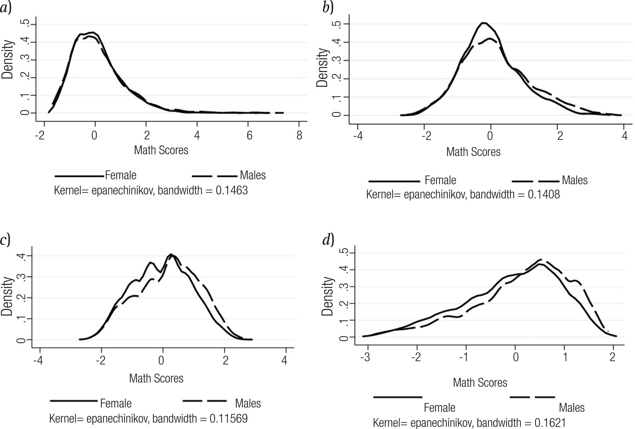
Outcome variable in this analysis is math test scores. ECLS-K measures students’ outcomes by test scores from direct cognitive assessment. The content area of the test is based on the NAEP (TOURANGEAU et al., 2006). Each test was adapted according to students’ age in order to make them appropriate for each grade. For this study, IRT test scores reported in the database were transformed to have mean zero and a standard deviation of one for the overall sample on each of tests and time periods, to allow for establishing comparisons with other studies that have used the same data set. Figure (1) presents the distribution of math for kindergarten, first, third and fifth grade. As observed, gender disparities are not pronounced, as a matter of fact at kindergarten differences are negligible, but the gap broadens as children progress in elementary school.
Source: prepared by the authors.
Fig 1. a. Test score distribution by gender and kindergarten. b. Test score distribution by gender and first grade. c. Test score distribution by gender and third grade. d. Test score distribution by gender and fifth grade.
Figure 1 Test score distribution by gender and grade
This study uses three types of variables that have been shown in the literature to have a strong correlation with children educational outcomes. These types of variables are related to children structural circumstances: parent´s educational attainment (categorical variable, with high school as reference), an indicator for whether the household is below poverty, an indicator for whether the family is a single-parent family and an indicator for whether the child attended Head Start3. Cultural variables included are: number of books at home, parent´s expectations of children educational attainment (getting a bachelor degree), whether parents consider if their children are better in math than their peers, an indicator for whether the mother suffers from depression and an indicator for whether the child is obese. The indicator of depression was constructed using two questions from parents´ questionnaire. Mothers were asked how often they felt depressed or sad during the previous week. We followed the depression scale developed by the center of epidemiologic studies. This variable was coded as one when mothers declared feeling sad or depressed a moderated amount of time and most of the times. Value of zero was given to responses of never – some of the time feeling sad or depressed. Child BMI was calculated based on weight and height provided by ECLS-K study. Children were measured at kindergarten (5 years old), first grade (6 years old), third grade (8 years old) and fifth grade (10 years old). To classify children as obese CDC´s standards are followed (if their percentile rankings were equal or greater to 95th: obese; between percentile 85th and 95th: overweight; between percentile 5th and 85th: normal). This variable takes the value of one if child is obese, zero otherwise. BMI was included given the growing literature that points to this phenomenon as related with disadvantaged household characteristics (SEALY, 2010; WELLS et al., 2010). Lastly, school variables included are: school type, class enrollment, teacher´s education, certification and experience in years. Variables used in this analysis come from parents, teachers and school administrator questionnaires provided in the non-restricted data set. To ensure that comparisons across waves are not affected by attrition, the analysis is restricted to a subsample of children who have math scores in kindergarten, first, third and fifth grades.
Table (1) presents the mean and standard deviation (in parenthesis) by grade and gender of the variables considered in this study. (*) indicates the mean is significantly higher than the mean of the variable for the opposite gender in the given grade at a 90% confidence level, (**) at a 95% confidence level, and (***) at a 99% confidence level. Generally speaking, the statistics show that students´ initial conditions at kindergarten remain constant as children progress through elementary school. There are no important differences in the proportion of males and females with parents holding at least a high school diploma. Females have a higher proportion of parents with a bachelor degree, whereas males’ parents report a higher rate on graduated schooling. Gender differences in parental education remain significant and constant throughout grades, suggesting that parents do not continue their studies at the time their children attend school. For other structural variables such as living below the poverty line and attending Head Start schools, there are no important differences. Nonetheless, more females than males live in single families, which is generally associated to worse outcomes at school (DOWNEY, 1994). In terms of structural variables, an overall glance at gender disparities indicates that males have better surrounding conditions than females. In the next section, it is analyzed whether such differences actually impact the students’ math performance.
Table 1 Descriptive statistics by gender
| Females | Males | |||||||
|---|---|---|---|---|---|---|---|---|
| Kindergarten | First | Third | Fifth | Kindergarten | First | Third | Fifth | |
| Structural variables | ||||||||
| Parent holds at least a high school diploma | 0.525 | 0.495 | 0.420 | 0.436 | 0.528 | 0.498 | 0.430 | 0.433 |
| (0.499) | (0.500) | (0.494) | (0.496) | (0.499) | (0.500) | (0.495) | (0.496) | |
| Parent holds at least a bachelor degree | 0.503** | 0.514* | 0.549** | 0.547* | 0.483 | 0.498 | 0.529 | 0.533 |
| (0.500) | (0.500) | (0.498) | (0.498) | (0.500) | (0.500) | (0.499) | (0.499) | |
| Parent holds at least a graduate degree | 0.084 | 0.086 | 0.105 | 0.110 | 0.095** | 0.097** | 0.116* | 0.119* |
| (0.277) | (0.281) | (0.307) | (0.313) | (0.293) | (0.296) | (0.320) | (0.324) | |
| Below poverty | 0.178 | 0.169 | 0.175 | 0.178* | 0.171 | 0.161 | 0.167 | 0.166 |
| (0.383) | (0.375) | (0.380) | (0.383) | (0.377) | (0.368) | (0.373) | (0.372) | |
| Time invariant | ||||||||
| Attended Head Start | 0.143 | 0.143 | 0.143 | 0.143 | 0.135 | 0.135 | 0.135 | 0.135 |
| (0.350) | (0.350) | (0.350) | (0.350) | (0.341) | (0.341) | (0.341) | (0.341) | |
| Lives in single family | 0.196** | 0.196** | 0.196** | 0.196** | 0.178 | 0.178 | 0.178 | 0.178 |
| (0.397) | (0.397) | (0.397) | (0.397) | (0.382) | (0.382) | (0.382) | (0.382) | |
| Whites | 0.582 | 0.582 | 0.582 | 0.582 | 0.592 | 0.592 | 0.592 | 0.592 |
| 0.493 | 0.493 | 0.493 | 0.493 | 0.492 | 0.492 | 0.492 | 0.492 | |
| Blacks | 0.110 | 0.110 | 0.110 | 0.110 | 0.111 | 0.111 | 0.111 | 0.111 |
| 0.313 | 0.313 | 0.313 | 0.313 | 0.314 | 0.314 | 0.314 | 0.314 | |
| Hispanic | 0.195 | 0.195 | 0.195 | 0.195 | 0.194 | 0.194 | 0.194 | 0.194 |
| 0.396 | 0.396 | 0.396 | 0.396 | 0.396 | 0.396 | 0.396 | 0.396 | |
| Asian | 0.055* | 0.055* | 0.055* | 0.055* | 0.048 | 0.048 | 0.048 | 0.048 |
| 0.227 | 0.227 | 0.227 | 0.227 | 0.214 | 0.214 | 0.214 | 0.214 | |
| Other | 0.058 | 0.058 | 0.058 | 0.058 | 0.055 | 0.055 | 0.055 | 0.055 |
| 0.233 | 0.233 | 0.233 | 0.233 | 0.228 | 0.228 | 0.228 | 0.228 | |
| Cultural variables | ||||||||
| Number of children books | 80.552 | 105.982 | 126.99*** | 111.27** | 80.262 | 102.658 | 115.775 | 104.284 |
| (71.263) | (130.009) | (196.241) | (181.071) | (122.780) | (164.631) | (158.396) | (165.897) | |
| Number of siblings | 1.453 | 1.503 | 1.541 | 1.547 | 1.468 | 1.530 | 1.564 | 1.553 |
| (1.135) | (1.126) | (1.131) | (1.147) | (1.130) | (1.125) | (1.131) | (1.101) | |
| Parent expectation on child’s future | 0.792*** | 0.792*** | 0.792*** | 0.792*** | 0.768 | 0.768 | 0.768 | 0.768 |
| (0.406) | (0.406) | (0.406) | (0.406) | (0.422) | (0.422) | (0.422) | (0.422) | |
| Child pays better attention than others | 0.882*** | 0.791*** | 0.834*** | 0.834*** | 0.798 | 0.726 | 0.743 | 0.743 |
| (0.323) | (0.406) | (0.372) | (0.372) | (0.401) | (0.446) | (0.437) | (0.437) | |
| Child solves problems better than others | 0.905*** | 0.815 | 0.842*** | 0.842*** | 0.869 | 0.806 | 0.811 | 0.811 |
| (0.293) | (0.388) | (0.365) | (0.365) | (0.337) | (0.395) | (0.392) | (0.392) | |
| Obese | 0.110 | 0.126 | 0.168 | 0.189 | 0.130*** | 0.137* | 0.193*** | 0.196 |
| (0.313) | (0.332) | (0.374) | (0.391) | (0.336) | (0.344) | (0.394) | (0.397) | |
| Mom’s depression | 0.072 | 0.078 | 0.078 | 0.078 | 0.082** | 0.076 | 0.076 | 0.076 |
| (0.259) | (0.267) | (0.267) | (0.267) | (0.274) | (0.265) | (0.265) | (0.265) | |
| School variables | ||||||||
| Teacher education | 0.363 | 0.709 | 0.409 | 0.425 | 0.349 | 0.723 | 0.408 | 0.418 |
| (0.481) | (0.454) | (0.492) | (0.494) | (0.477) | (0.448) | (0.492) | (0.493) | |
| Teacher experience | NA | 14.870 | 15.077 | 14.420 | NA | 14.866 | 15.104 | 14.490 |
| NA | (10.134) | (10.255) | (10.255) | NA | (10.157) | (10.217) | (10.254) | |
| Teacher certification | 0.638 | 0.089 | 0.098 | 0.896 | 0.645 | 0.082 | 0.094 | 0.897 |
| (0.481) | (0.285) | (0.298) | (0.305) | (0.479) | (0.274) | (0.292) | (0.304) | |
| Class enrolment | 20.681 | 21.17*** | 21.372*** | 22.744*** | 20.555 | 20.993 | 21.109 | 22.432 |
| (4.526) | (4.502) | (4.247) | (5.863) | (4.575) | (4.333) | (4.102) | (5.995) | |
| Public school | 0.792 | 0.797 | 0.807 | 0.814 | 0.800 | 0.805 | 0.814 | 0.819 |
| (0.406) | (0.402) | (0.395) | (0.389) | (0.400) | (0.396) | (0.389) | (0.385) | |
Source: prepared by the authors.
Note: variable mean by gender and grade in the full sample of students. Standard deviation in parenthesis. (*) indicates the mean of the variable is higher than the mean of the variable for the opposite gender in the given grade at a 90% confidence level, (**) at a 95% confidence level, and (***) at a 99% confidence level. Authors’ calculations.
Regarding cultural variables, relevant differences between males and females are reported for the number of children books, parents’ expectations about their children’s future, parents’ perception of whether their children pay better attention than others and solve problems better than others, and obesity indicator. For the first variable, female students have more children books than males by the time they reach third and fifth grade. Parents’ expectations and perceptions are also systematically higher for female students than males, while the proportion of male students with obesity is higher than the proportion of females. In terms of cultural variables, the environment surrounding female students tends to favor them over males. Gender disparities in cultural and family backgrounds have also been found in the literature (BUCHMANN; DIPRETE, 2006; ECCLES et al., 1990).
Finally, in the case of school-related variables, there are small but significant differences in class enrollment (about one or two additional students) that favor males.
Two empirical analyses are conducted in this paper: longitudinal and cross-sectional. The former is used to provide a big picture of gender differences in elementary school, providing information on three components: i) socioeconomic status (structural variables); ii) home practices, beliefs and expectations (cultural variables); and iii) general school conditions (school variables). Cross-sectional analysis is aimed at decomposing the achievement gap by gender. In this analysis we provide insight on the drivers on educational outcomes.
For the longitudinal analysis, the data is pooled and a regression analysis is conducted using longitudinal weights, primary sampling units and strata variables (TOURANGEAU et al., 2006). To focus on characterizing variations in math test scores, a linear specification is used as follows:
Where i indexes children, k indexes schools and t indexes grades. Dik is a vector of demographic characteristics, Titk is a vector of structural variables, Citk is a vector of cultural variables, and Ptkis a vector of school-level variables. The term δk is a fixed effect that captures unobserved variations between schools but remains constant between children and grades. Finally, ɛijk is the random error term that is specific to each child in grade t and school k.
Cross-sectional analysis consists of a nonparametric decomposition of race and gender gaps into four additive components following Ñopo (2008). Formally, the gender gap can be described as:
This specification follows Garcia, Ñopo & Salardi (2009).
Δx: Part accounted by differences between the distribution of males´ and females´ individual characteristics over their common support.
Δf: Due to the existence of some combinations of females´ characteristics that are not comparable to those of males.
Δm: Due to the existence of some combinations of males´ characteristics that are not comparable to those of females.
Δ0: Part that cannot be explained by differences in observable individual characteristics.
The Ñopo decomposition technique overcomes a difficulty of the traditional Oaxaca-Blinder (OB) approach. The OB uses a linear regression that faces the potential problem of misspecification due to extrapolation, namely, assuming that for every male there is at least a female counterpart with similar covariates (or viceversa), and thus their outcomes can be comparable. Briefly, the matching technique as explained in Garcia, (GARCÍA; ÑOPO; SALARDI, 2009) works in 5 steps. Firstly, a female is selected from the sample (without replacement). Secondly, all males that have the same characteristics as the previously selected female are selected. Thirdly, with all the individuals in the second step, it was selected a synthetic individual whose characteristics are equal to the average of all of them and then he was “matched” to the original female created. Fourthly, the observations of both individuals (the synthetic male and the female) are put in their respective new samples of matched individuals. This process is repeated until the original female sample is exhausted. In the end a new dataset containing observations of “matched females”, “matched males”, “unmatched females” and “unmatched males” is created, so that the sets of matched males and females have the same empirical distributions of probabilities for the selected characteristics (ÑOPO, 2008). A detailed explanation of the method is available in Ñopo (2008).
Results
As a first attempt to understand the factors driving the divergences in test scores between males-females during elementary school, we explore the contribution of different variables to the average achievement gap. We use longitudinal data, pooling four waves of data collection: kindergarten, first, third and fifth grades, and restrict the analytical sample to children who have complete information on all variables and grades used in the analysis.
Table (2) shows the evolution of the gender gap from kinder to fifth grade. These estimations are made in the cross-section of students at each grade and they all include school fixed effects, race indicators, structural variables, cultural variables, and school-related variables. The gender gap is significant and consistent across grades and increases as children go through elementary school. During kindergarten, the gender gap is almost negligible. Males score 0.096 standard deviations above females. However, once in first grade the gap increases by 130% and males outperform females by 0.22 standard deviations. During third grade, the gap broadens even further and there is a difference of 0.27 standard deviations in the math scores of males and females. Finally, during fifth grade the gap reduces by 0.036 standard deviations. The overall increase in the gender gap from kinder to fifth grade is 142%. The variation in the number of observations per grade has to do with missing values in several covariates.
Table 2 IRT math score gender gap by grade
| Dependent variable: IRT math scores | ||||
|---|---|---|---|---|
| Kinder | First | Third | Fifth | |
| Female | -0.0960*** | -0.221*** | -0.268*** | -0.232*** |
| (0.0215) | (0.0228) | (0.0228) | (0.0269) | |
| Controls | ||||
|
|
||||
| Race | Yes | Yes | Yes | Yes |
| Structural | Yes | Yes | Yes | Yes |
| Cultural | Yes | Yes | Yes | Yes |
| School | Yes | Yes | Yes | Yes |
|
|
||||
| Observations | 7,096 | 6,304 | 6,154 | 4,455 |
| R-squared | 0.096 | 0.108 | 0.181 | 0.206 |
| Number of schools | 802 | 881 | 1,077 | 1,117 |
Source: prepared by the authors.
Note: IRT math score gender gap by grade. The first column corresponds to first grade, the second column to third grade and the third column to fifth grade. The specifications include all structural, cultural and school variables, and school fixed effects. Robust standard errors in parenthesis. *** p<0.01, ** p<0.05, * p<0.1.
Table (3) presents the estimation of the conditional average math test score in the panel of students, which is assumed to be linearly related with the covariates used in the analysis. First and second columns present the results for females and males, respectively, while third column shows the results for the full sample. Third column shows that even after conditioning on grade and school, after ruling out the unobserved heterogeneity between schools and grades, there is a significant math score gap of 0.239 standard deviations between males and females, favoring males. In terms of race, it was found that Blacks score 0.484 standard deviations below and Hispanics score 0.250 standard deviations below Whites (reference category). This goes in line with some of the related literature (JENCKS; PHILLIPS, 1998; HEDGES; NORWELL, 1999; MCDONOUGH, 2015). Math IRT scores of Asians, on the other hand, do not differ systematically from those of white students.
Parents´ education has a strong and positive correlation with children scores for both males and females, as well as the number of children books at home, parents’ expectations of child future (finishing college) and parents´ perception of their children paying attention and solving problems better than others. By contrast, children living in poverty do worse on test scores. Interestingly, attending Head Start program has a negative effect on females test scores, but the correlation does not hold in the case of males. Marsh et al. (2002) also find academic self-concept factors to be significantly correlated with achievement test scores while nonacademic factors are insignificant as we show ahead.
Table 3 Estimation of the conditional average math test score in the panel sample
| Females (1) | Males (2) | All (3) | |
|---|---|---|---|
| Female | -0.239*** | ||
| (0.0197) | |||
|
|
|||
| Race | |||
| Blacks/AA | -0.538*** | -0.508*** | -0.485*** |
| (0.0706) | (0.0830) | (0.0497) | |
| Hispanics | -0.200*** | -0.270*** | -0.251*** |
| (0.0464) | (0.0582) | (0.0361) | |
| Asians | 0.00715 | 0.104 | 0.0520 |
| (0.0798) | (0.110) | (0.0630) | |
| Other | -0.198* | -0.0638 | -0.123* |
| (0.0792) | (0.0840) | (0.0516) | |
|
|
|||
| Structural variables | |||
| Parent holds at least a bachelor degree | 0.229*** | 0.130*** | 0.169*** |
| (0.0343) | (0.0335) | (0.0215) | |
| Parent holds at least a graduate degree | 0.364*** | 0.251*** | 0.328*** |
| (0.0520) | (0.0522) | (0.0336) | |
| Below poverty | -0.179*** | -0.162*** | -0.163*** |
| (0.0385) | (0.0449) | (0.0271) | |
| Attended Head Start | -0.126* | -0.0754 | -0.117** |
| (0.0499) | (0.0530) | (0.0371) | |
| Lives in single family | -0.0305 | -0.0144 | -0.0212 |
| (0.0357) | (0.0451) | (0.0252) | |
|
|
|||
| Cultural variables | |||
| Number of children books | 0.000210** | 0.000180** | 0.000215*** |
| (0.0000749) | (0.0000603) | (0.0000462) | |
| Number of siblings | -0.00705 | 0.0142 | 0.00413 |
| (0.0127) | (0.0134) | (0.00828) | |
| Parent expectation on child’s future | 0.185*** | 0.133*** | 0.165*** |
| (0.0357) | (0.0360) | (0.0243) | |
| Child pays better attention than others | 0.180*** | 0.166*** | 0.171*** |
| (0.0392) | (0.0339) | (0.0238) | |
| Child solves problems better than others | 0.526*** | 0.596*** | 0.591*** |
| (0.0444) | (0.0415) | (0.0287) | |
| Obese | -0.0363 | -0.0490 | -0.0413* |
| (0.0271) | (0.0293) | (0.0195) | |
| Mom’s depression | -0.123* | 0.0764 | -0.0385 |
| (0.0548) | (0.0529) | (0.0360) | |
|
|
|||
| School variables | |||
| Teacher education | 0.0362 | -0.0283 | 0.00664 |
| (0.0213) | (0.0198) | (0.0159) | |
| Teacher experience | -0.00134 | -0.000446 | -0.000710 |
| (0.000931) | (0.00104) | (0.000766) | |
| Teacher certification | -0.0389* | -0.0213 | -0.0408** |
| (0.0174) | (0.0183) | (0.0130) | |
| Class enrollment | 0.00799** | 0.0134*** | 0.0122*** |
| (0.00274) | (0.00291) | (0.00219) | |
| Public school | -0.105 | -0.197 | -0.115 |
| (0.119) | (0.167) | (0.0912) | |
| School fixed effects | YES | YES | YES |
| N | 8544 | 8369 | 16913 |
| Number of schools | 1108 | 1075 | 1353 |
Source: prepared by the authors.
Notes: The dependent variable in this model is the IRT math score.
Excluded category in race is white students.
Bootstrap standard errors in parentheses. ***p<0.01, **p<0.05, *p<0.1.
Amongst the variables at school level, only class enrollment is significantly related to children’s outcomes. Higher class enrollment explains an increase of 0.012 standard deviations in math scores. Although the magnitude of the effect is small, the positive sign of the coefficient may seem counterintuitive. Nonetheless, this result is consistent with the idea that in competitive environments academic performance shows a different trend when compared to less competitive environments. Niederle & Vesterlund (2010) show that males perform better than females in competitive settings, so males may drive the effect that we are capturing.
Gap decomposition
The evidence presented so far indicates that gender gaps in math are driven by socioeconomic conditions. However, despite explaining large variations in test scores, there is a remaining unexplained gap. This may indicate that the gender achievement gap could be explained by misspecification due to extrapolation. The Ñopo decomposition used in this section explores how important such effect is. In order to control for year-specific unobservables the gap decomposition is estimated for each grade.
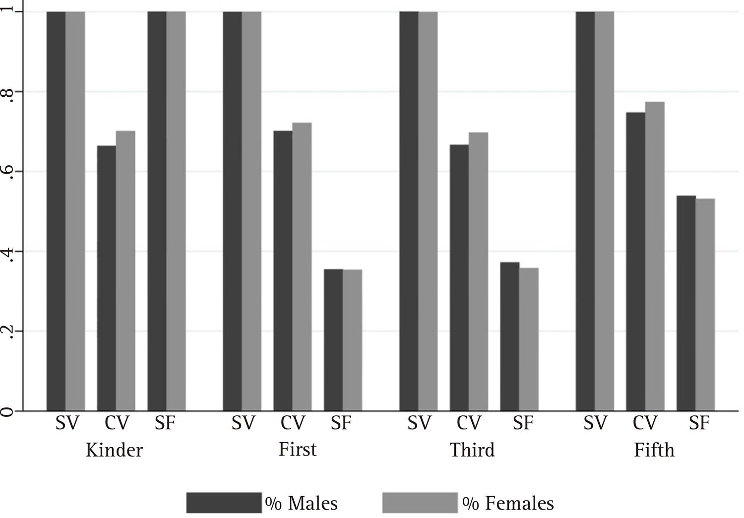
Figure (2) and Table (4) show the common support in the non-parametric matching and the decomposition of the gender gap for each grade, respectively. The structural variables are the first group of variables over which the gap is computed. Then cultural variables and finally school variables are added. In the matching process during kindergarten, first, third and fifth grade over structural variables, 100% of males and females fall in the common support. When cultural variables are added, 20% of the observations are lost. For example, during first grade after cultural variables there are 70% of males and 72% of females in the common support. The inclusion of school factors increases the common support during kindergarten, but reduces it around 20% during first, third and fifth grade.
Table 4 Gender gap decomposition
| SV | +CV | +SF | |
|---|---|---|---|
| Kindergarten | |||
|
|
|||
| Gap | -0.0399 | -0.0399 | -0.0399 |
| Delta O | -0.0302 | -0.0757 | -0.0399 |
| (0.0158) | (0.0194) | (0.0146) | |
| Delta M | 0.0003 | 0.1581 | 0.0000 |
| Delta F | 0.0002 | -0.1363 | 0.0000 |
| Delta X | -0.0103 | 0.0140 | 0.0000 |
| % M | 0.9994 | 0.6641 | 1.0000 |
| % F | 0.9996 | 0.7011 | 1.0000 |
|
|
|||
| First grade | |||
|
|
|||
| Gap | -0.1175 | -0.1175 | -0.1175 |
| Delta O | -0.1082 | -0.1486 | -0.0590 |
| (0.0148) | (0.0180) | (0.0230) | |
| Delta M | 0.0001 | 0.0966 | -0.2005 |
| Delta F | 0.0000 | -0.0779 | 0.1396 |
| Delta X | -0.0095 | 0.0124 | 0.0024 |
| % M | 0.9996 | 0.7013 | 0.3546 |
| % F | 0.9996 | 0.7210 | 0.3536 |
|
|
|||
| Third grade | |||
|
|
|||
| Gap | -0.1805 | -0.1805 | -0.1805 |
| Delta O | -0.1724 | -0.1994 | -0.1371 |
| (0.0206) | (0.0171) | (0.0219) | |
| Delta M | 0.0000 | 0.1087 | -0.1387 |
| Delta F | -0.0001 | -0.1039 | 0.0942 |
| Delta X | -0.0079 | 0.0142 | 0.0012 |
| % M | 1.0000 | 0.6662 | 0.3719 |
| % F | 0.9989 | 0.6971 | 0.3576 |
|
|
|||
| Fifth grade | |||
|
|
|||
| Gap | -0.1890 | -0.1890 | -0.1890 |
| Delta O | -0.1780 | -0.2216 | -0.2116 |
| (0.0143) | (0.0166) | (0.0174) | |
| Delta M | 0.0003 | 0.0706 | -0.0521 |
| Delta F | 0.0000 | -0.0560 | 0.0739 |
| Delta X | -0.0114 | 0.0179 | 0.0008 |
| % M | 0.9998 | 0.7470 | 0.5390 |
| % F | 1.0000 | 0.7738 | 0.5312 |
Source: prepared by the authors.
Note: non-parametric gender gap decomposition. The first column controls for structural variables (parents’ education, below poverty, attended Head Start, single family), the second adds cultural variables (number of books at home, number of siblings, parents’ expectations, parents’ perception of child’s abilities, obese, mom’s depression), and the third adds school factors (teacher education and certification, class enrollment, school type). Standard error in parenthesis.
Table (4) shows the decomposition of the gender gap. Delta O accounts for the unexplained portion of the gap. Delta F shows the part of the gap that is explained by females’ intrinsic characteristics, Delta M by males’ intrinsic characteristics, and Delta X shows the part of the gap that is explained by characteristics that are common between both groups.
The first column of table (4) controls for sociodemographic variables, the second column adds cultural variables and the third one includes school factors. These results confirm that the gender gap increases gradually as children progress through elementary school. Although the finding was presented earlier in a linear regression, in such scenario the results could have been biased because of the math scores of children that have no match in their structural, cultural, and school backgrounds. Using the non-parametric matching to decompose the gap, we account for not-matched factors focusing only in males and females who fall in the common support, in other words who have the same structural, cultural, and school characteristics. The gap goes from -0.04 standard deviations in kindergarten favoring males over females, to -0.1175 in first grade, to -0.1805 in third grade, and ends in -0.1890 in fifth grade. Overall, the magnitude of the gap decreases compared to the one presented in the linear regression, which suggests that the previous results were probably biased. To the best of our knowledge, no study so far has accounted for not-matched factors and this is the main contribution of this analysis to the literature of gender achievement gaps during elementary school.
The importance of structural variables in explaining the gap also decreases as children progress through elementary school. In kindergarten, they account for 34% of the gap, 8% during first grade, 4% during third grade, and 6% during fifth grade. In the second column with cultural variables, the unexplained portion of the gap increases in absolute value, going from -0.0302 to -0.0757 in kinder, from -0.1082 to -0.1486 in first grade, from -0.1724 to -01994 in third grade, and from -0.1780 to -0.2216 in fifth grade. Females’ structural intrinsic characteristics had no effect on the math score disparities; when cultural variables are added to the distribution of female characteristics, however, they start disfavoring them over males as noted in the Delta F component. When the last group of variables is included, results show, first that unexplained portion of the gap decreases; second that males’ intrinsic characteristics associated to the schools they attend disfavor them over females but the effect is not sufficient to put males in lower tails of the math score distribution; and third that in general, the explained portion of the gap decreases.
In sum, gender gaps increase progressively in elementary school, at kindergarten differences they are negligible; however, by fifth grade they are significant and favor males over females. Between first grade (0.1175) and fifth grade (0.1890) the gap increases by 60.8%. The evidence presented in this analysis suggests that gender gaps grow rapidly and no single set of variables included in the analysis explains an important portion of the gap. Hence, unobserved factors (beyond SES and standard school outputs) play a major role on explaining gender differences on educational outcomes.
Discussion
Explaining achievement gaps and identifying factors that may affect children’s educational outcomes is a complex task. Most of the complexity of this kind of research is that educational outcomes are the product of an intricate interaction of several structural factors: family conditions, school quality and public policies. Mostly because of data limitations, empirical analysis has been unable to control for all family and school influences on educational outcomes, and it is unlikely that statistical adjustments relying only on measured school and family variables can account completely for students’ performance (HANUSHEK; RIVKIN, 2009).
Summarizing, it was found that gender gaps increase significantly over elementary school. The unexplained components of the math gender differences increase over time, which suggests that as children progress over their schooling years, the importance of observed factors such as socioeconomic conditions decreases. Observable individual socioeconomic characteristics explains little. In first grade, socioeconomic variables explain 8% of females-males differences but by third and fifth grade socioeconomic circumstances explain less than 6% of such differences. This implies an important question in terms of policy formulation. Much of program implementation in education, like Head Start and No Child Left Behind are aimed at leveling socioeconomic disparities, which are relevant in the case, for instance, of racial gaps where socioeconomic conditions explain an important share of educational outcomes (i.e. comparing white children with Hispanic or Blacks) (JENCKS; PHILLIPS, 1998; HEDGES; NORWELL, 1999; McDONOUGH, 2015; FRYER; LEVITT, 2004, 2006). However, in the case of gender, establishing policy implementation could become more challenging since it is more difficult to establish what the mechanisms are behind gender test scores gaps.
The pace at which gender gaps evolve is worrisome. In kindergarten, although differences between males and females in math test scores were significant they were small in magnitude, but between first and fifth grades, the gender gap increases by 60.8%. This is a finding that deserves further research attempted at explaining why such a significant difference evolves and what factors may be associated with it. Disparities in socioeconomic conditions have been the usual suspect on explaining differences in educational outcomes. However, in the case of gender, it seems there are other unobservable factors playing a major role.
Results of the gender gap decomposition show that school factors are not relevant for explaining differences in math test scores –at least with the variables used in the model. The portion of the gap that is explained by observable characteristics once controlling for school factors is still relatively small, it does not exceed 3 percentage points at any grade. Baseline panel estimations using within-school differences in the observables (school fixed effects) also suggest that school factors are not significant for explaining the variations in math test scores, except for class enrollment. A caveat needs to added to this point, however: school level characteristics were not significantly different at any point in the time analyzed, which did not provide variation in the model.
The methodology allowed to identify which part of the gap was due to characteristics that are unique to males and females. The effect varies by grade and by specification and is a warning to researchers in the sense that the published gaps may be underestimated or overestimated. This is an area of research that merits further analyses. Decomposing the gap using Ñopo’s non-parametric technique allows to compare individuals who are similar both in their observable and unobservable characteristics yielding a better estimation of gender gaps. This methodology controls for outliers in the sense that the gap and its decomposition are estimated only over the individuals that lie within the region of common support, limiting extrapolation. We were unable to capture measures on quality of education, school materials, and participation in subsidy programs that might affect income, child and mom’s age to capture non-linear effects on achievement, which could be important sources of variation.

