


 Inglés (pdf)
 Articulo en XML
 Enviar articulo por email
 Permalink
1 Introduction
The Brazilian National Education Plan (PNE) 2014-20241 advocates the necessity of providing “full-time Education in at least 50% (fifty percent) of the public schools to attend at least 25% (twenty-five percent) of the students from the basic level of Education” (free translation).
The Brazilian Federal Government, by Provisional Measure (MP) nº 7462, converted into law nº 13,4153, created a policy to increase the number of full-time public schools in the country. It established that Brazilian states would offer full-time schooling, finding the best model to adopt - considering the local context - to increase the number of students and schools with extended journeys.
Even with some particularities (Araújo et al., 2020; Battistin and Meroni, 2016; Castanho and Mancini, 2016; Fukushima, Quintão and Pazello, 2002; ; ; show that the full-time schooling policy positively affected students’ scores on a standardized test in mathematics and language. In a general approach, increasing time in school works as a tool for schooling effectiveness (; ; ; igal, 2022).
It is, however, important to notice the existence of a trend to represent full-time schools as the salvation for Education, mixing the right that low-income families have to quality Education and a comprehension that full-time schools have no contradictions or externalities on Education systems (Castanho and Mancini, 2016).
In the same path, Silva and Jófili (2022) say that the dominant discourse about quality in Education associates good Education and good performance in standardized tests, concealing other meanings of quality and reinforcing the perspective of a salvationist full-time Education since it tends to produce better results.
In the Brazilian case, full-time schools tend to attract a homogeneous profile of students since the socioeconomic profile and demographic characteristics significantly impact school choice (Bae; Cho; Byun, 2019; Costa; Kolinski, 2012; Koslinski; Alves; Lange, 2013). Students with work obligations and social vulnerability tend to face difficulties attending full-time schools (Vieira et al., 2016).
Moreover, Alves and Soares (2013) show that infrastructure conditions and the institutions’ complexity positively correlate with better results in standardized test scores and that students with less privileged socioeconomic backgrounds tend to exhibit lower score results. Also, Bellei (2009) argues that full-time programs have more significant positive effects on scores of rural students, students who attended public schools, and students situated in the upper part of the distribution of the scores.
In his analysis, Fernandes (2019) states that high-stakes standardized test scores can promote negative externalities in the Education system, related to: a) reduction of curriculum to what appears in the tests; b) the school administration may direct the use of strategies to remove students who are not performing as expected or perceived as a performance risk on standardized test scores; c) focus on students classification and ranking. Rostirola (2021) points out that not only the use of high stake standardized test scores but the system of accountability may result in gaming and ineffective regulation, with an intense charge on results and the teachers being accountable for results not directly connected to their actions.
Although socioeconomic inequality analysis is very relevant, it is also essential to reflect on the relationship between schooling effectiveness and inequality, understood as the dispersion of the effectiveness among the unities. Usually, increases in the effectiveness of an Education system (measured by standardized test scores) tend to happen centered on schools of a specific type, schools under similar conditions, or even schools that already have higher scores (Bellei, 2009). The full-time implementation for specific students could mean that the inequality between them and those in regular part-time schools will increase.
Kuznets Curve – CK (Kuznets, 1955) offers a way to comprehend the relationship between effectiveness and inequality. Based initially on countries’ economic growth and income concentration, CK describes an inverted U-curve correlating these two variables. In the first moment, economic growth increases economic inequality and decreases after a threshold point.
With a focus on schooling expansion and inequality level, Ram (1990) points to a complex relationship between the level of Education of the individuals measured by years of educational attainment (schooling effectiveness) and the measures of dispersion of this educational attainment (schooling inequality)4. Increasing the individual Education level negatively impacts the educational system’s inequality level until a critical point where inequality starts to decrease, and the educational level works as a tool to reduce inequality.
Many authors have revisited the CK from different perspectives, observing variations on the “U shape”. The relationship between happiness and inequality (Ram, 2017) has a U-inverted shape; the level of development and income inequality in the United States has a relationship in a regular-U shape (Blanco; Ram, 2019); the relationship between per capita income growth and inequality in Brazil tends to an inverted-u shape only for those up to a specific income (Linhares et al., 2012); the relationship between the average schooling level and schooling dispersion may assume an inverted-U shape when dispersion is measured in terms of standard deviation, and a regular-U shape when using the Gini coefficient (Shukla; Mishra, 2019).
Neves and Almeida (2016) have incremented Ram’s analysis (1990), adapting Kuznets’s (1955) hypothesis, adopting the city as the unit level, the Prova Brasil5 as the efficiency index, and socioeconomic variables6 as control. They found that the relationship between increasing effectiveness and inequality has a regular-U shape. Due to the small magnitude of the effect of the quadratic term of proficiency, the relation could even be considered linear (monotone and negative).
This paper aims to analyze the relationship between schooling effectiveness and schooling inequality in Pernambuco, Brazil, using state standardized tests to investigate the relationship between full-time journeys and inequality, incrementing the analyses made by Neves and Almeida (2016) with a focus on full-time schools and specific characteristics of the schools and using control variables that vary across time and others that are stable over time. We used the age-grade distortion index as a control, since the more significant the dispersion in terms of age in the classroom, the lower the average proficiency (Portella; Bussmann; Oliveira, 2017).
Regarding the analyzed data, Prova Brasil imposed some limitations on the panel analysis, since it is biannual. Alternatively, we used annual data of the 12th-grade level from the Sistema de Avaliação Educacional de Pernambuco (Saepe) (Educational Assessment System of Pernambuco), from the Board of Education and Sport from the State of Pernambuco (SEE-PE), and data from Pernambuco at Censo da Educação Básica (the census of primary Education) between 2008 and 20217.
SAEPE is Pernambuco State ow educational system to evaluate all senior students at the primary level. The exam follows Item Response Theory (IRT) and occurs annually, involving 9th-grade and 12th-grade students with Portuguese Language and Mathematics items. It is a simulation and monitoring strategy for the Basic Education Assessment System (Saeb)8, and to the Programme for International Student Assessment (Pisa).
The focus on Pernambuco’s case is because of its extensive process of implementing full-time schools, which, starting in 2008, reached the universalization of municipal provision in 2016. The public school system has four types of schools according to the extension of the school day: Integral (schools with a five days full-time journey), Regular (part-time schools with no extended days), partial (schools with three days of full-time journey), and technical full-time school (technical high schools with five days full-time journey that combines propaedeutic and technical subjects).
This paper has the following structure: i) presentation of the research method, including Automated Exploratory Data Analysis - autoEDA theory and practice and panel data analysis theory and practice; ii) analysis description, with data preparation, autoEDA, and schooling inequality using panel data analysis, including model selection and outcomes; iii) discussion of the findings, focusing on the shape of the relationship between effectiveness and inequality, and exploration of the uniform variables and varying over time variables that relate to the inequality; iv) conclusion, presenting data and study limits, and possibilities for future work.
2 Research Method
In this study, we used panel data: the same individuals have a set of attributes repeatedly measured in different periods/times (Mesquita; Fernandes; Figueiredo Filho, 2021). In our case, data from Pernambuco State (Brazil) public high school institutions, on standardized tests, from 2008 to 2021, aggregated by development region9 of Pernambuco.
With the original dataset, we performed a process of Automated Exploratory Data Analysis - autoEDA. It involves using specific computer packages, libraries, or programs to accelerate or even automate the actions of data description and quality verification, using summaries and data visualization to understand the set better (Staniak; Biecek, 2019).
We executed the autoEDA using R, RStudio, and the funModeling package (Casas, 2019, 2023), in three steps: (i) quality verification for the proportion of zeros, not available, type, unique values, and wrong imputation, (ii) categorical variables numeric and visual analysis of frequency and distribution, (iii) numeric variables analysis of central tendencies, and et cetera.
Considering that unbalanced panels are suited to bias if the information gap is systemic (Mesquita; Fernandes; Figueiredo Filho, 2021), it was necessary to do specific tests to observe if data were missing (or not) at random (Kabacoff, 2011).
Since our panel data related numeric variables (age-grade distortion and standardized test scores) with categorical (type of institution, duration of journey), we chose a correlation method to evaluate if missing values were systemic. For example: would it be that age-grade distortion was not available for rural schools? If we detect a correlation between missing values on age-grade distortion and rural schools (or any specific association), it would indicate that data were not missing randomly.
Using the shadow matrix correlation technique - in which the rows are the variables and the columns represent the missingness - it is possible to identify if data is missing/not missing at random, by observing the relation between rows and columns (Kabacoff, 2011). The process showed that data were missing randomly.
After aggregation, the final dataset remained cross-section dominant but with a lower n (16) and changed from unbalanced to balance since the number of regional offices of Education did not change. We performed a panel regression with the final dataset, a balanced and cross-section dominant panel, using R, RStudio, and the plm package (Croissant; Millo, 2008, 2018).
Panel regression is a modification of the traditional linear regression Yi = 𝛼 + 𝛽1Xi1 + … + 𝛽pXip + 𝜀i, in which (i) the time component “t” is added, and (ii) the composite error “𝜀” is broken into fixed error “𝜇i” and variable error “𝜈it”, resulting in Yit = 𝛼 + 𝛽1Xit1 + … + 𝛽pXitp + 𝜇i + 𝜈it (Croissant; Millo, 2008, 2018; Mesquita; Fernandes; Figueiredo Filho, 2021).
Since panel regression combines units and times, it may fall under time series problems (like serial correlation) or sectional problems (such as cross-sectional dependence) and is also related to linear model assumptions (no perfect collinearity, for example) (Mesquita; Fernandes; Figueiredo Filho, 2021).
We created the panel regression model following the contributions present in Colonescu’s (2016), Croissant and Millo’s (2008, 2018), and Mesquita, Fernandes and Figueiredo Filho, (2021) works. That is, we estimate four regressions using the basic panel model methods: (i) pooled, (ii) first differences - FD, (iii) fixed effects - FE, and (iv) random effects - RE.
The first method (pooled) is close to the traditional estimation of a linear model since no specific characteristics of units are considered, and it expects that independent variables have all the relevant information, resulting in only one intercept “𝛼” and the undivided error “𝜀”.
The second method (FD) is best used with panels with time problems because subtracting the previous period reduces serial correlation and non-stationarity; and reduces variability and available information.
With the third (FE), the effects of the independent variables are fixed, regardless of the unit (in this case, gre), while the intercept is different for each unit. It is essential to say that FE can be considered the standard variation for panel data since it focuses on the variable aspects of units (Croissant; Millo, 2018; Mesquita; Fernandes; Figueiredo Filho, 2021).
Finally, the last method (RE) considers that the effects of the independent variables are random, changing for each unit and time, which results in 𝜇i and 𝜈it being perceived as stochastic and not related to the independent variables, resulting in models that retain information from variables that are constant in the panel.
To choose an acceptable method, we followed the Croissant and Millo (2008) and Mesquita, Fernandes and Figueiredo Filho (2021) recommendations:
Pooled vs. FE: analyze the intercepts distribution and use F-test, with the null hypothesis being that there are no significant effects (i.e., pooled is adequate);
Pooled vs. RE: Breusch-Pagan test, observing if (null hypothesis) unit-specific variance is zero (i.e., pooled is adequate);
FE vs. RE: Hausman test, that indicates if (null hypothesis) the unobserved variation from units is unassociated with the regressors. In case of an association, only FE estimators will be consistent; in case of the absence of association, both models, FE and RE, are consistent;
FD vs. FE: Wooldridge first–difference–based test. Choosing FD or FE as a null hypothesis makes it possible to understand which method is more efficient. It is also essential to analyze the overall fit and regression metrics such as R2.
Once the model is selected, it is necessary to test for (i) normal distribution of errors, (ii) serial correlation in the error term (not needed for RE), and (iii) cross-sectional dependence since events may occur and change all 12 development regions dynamics. It is possible to use robust variance-covariance matrix methods to address these problems and produce robust estimators (Beck; Katz, 1995; Driscoll; Kraay, 1998; Zeileis; Hothorn, 2002).
3 Materials and Results
In this section, we present the analysis description, divided in three steps: i) data preparation, including data cleaning and aggregation ; ii) autoEDA, exploring data patterns and data quality; and iii) the panel data analysis of schooling inequality, with model selection and outcomes.
3.1 Data preparation
The dataset used in this study was collected through the Public Transparency Portal of the SEE-PE (process nº 57419/2022 and process nº 60776/2023). The available variables were: (1) the year of the test; (2) school code; (3) school name; (4) the type of journey, according to the extension of the school journey (five days full-time school, three days full-time school, part-time school, full-time technical school); and (5) schools Idepe. With these variables, we also created (6) the Idepe (Idepe2) quadratic term and the standard deviation of the Idepe.
We merged school information from the census of primary Education into the original data: (7) the school’s city name, (8) the city’s code on a national base, (9) the name of the regional educational office, (10) the development region, (11) the school city’s localization (rural or urban), (12) the proportion of age-grade distortion from the 12th-grade students, (13) school with internet dummy, (14) school with night classes dummy, (15) school with classes for adults dummy, (16) total of students, (17) a total of female students, (18) a total of white students.
Following Neves and Almeida (2016) and Ram (1990), it was necessary to aggregate data to generate the proxy for inequality - standard deviation of the standardized test score, which entered the model as the dependent variable, since (i) the standard deviation was not available for schools, and (ii) the unbalanced data panel could increase bias (Mesquita; Fernandes; Figueiredo Filho, 2021).
It is important to remember that Neves and Almeida (2016) aggregate data by city. However, when we analyze data from 12th-grade students, the states fund and manage high schools in Brazil. Also, this aggregation is impossible, considering that many cities have only one high school.
Before aggregation (original dataset), the panel was cross-section dominant and unbalanced (Mesquita; Fernandes; Figueiredo Filho, 2021), i.e., the measures were not available for all individuals in all periods - unbalanced - and the number of individuals was more significant than the number of periods (n>T) - cross-section dominant.
Finally, after aggregation by development region, we merged the previous school data with the city’s (19) GDP and (20) population. We created the variables (21) GDP per capita, (22) the populational rate of schools with a five days full-time journey, (23) the populational rate of schools with a part-time journey, (24) the populational rate of schools with three days full-time journey, (25) populational rate of full-time technical schools, (26) populational rate of schools with night classes, (27) populational rate of urban schools, (28) populational rate of schools with internet access, (29) populational rate of schools with classes for adults. The final database was analyzed through the autoEDA method, focusing on quality verification and pattern identification.
3.2 AutoEDA
Firstly, we observed if the values were missing at random, using shadow matrix correlation. This technique isolates missed values and then observes if these values correlate with the other variables. In the present case, we verify that the correlation had low values (between -0.27 and + 0.16), showing that the values were missing at random and had no specific relation with the variable’s values. Excluding the missing values, corresponding to 8.5% of the original data, was possible.
Secondly, we analyzed the trajectory of Schooling Effectiveness and Schooling Inequality using the Idepe and its standard deviation. Figure 1 shows the overall mean, and the lower and upper limits of Idepe, and Figure 2 shows the standard deviation of the Idepe, both for all 12 development regions, from 2008-2021.
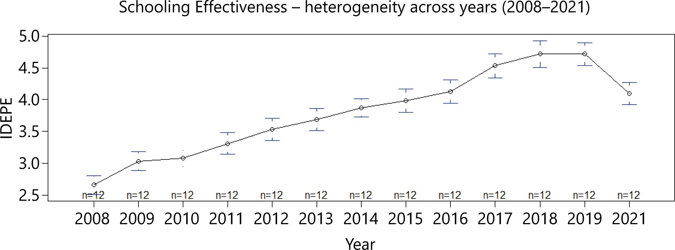
Source: Own elaboration (2024)
Figure 1 The overall mean and the lower and upper limits of Idepe for Pernambuco’s all 12 development regions from 2008-2021
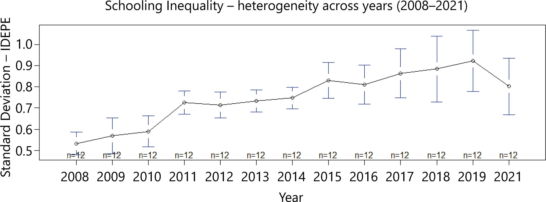
Source: Own elaboration (2024)
Figure 2 The standard deviation of the Idepe for Pernambuco’s all 12 development regions from 2008-2021
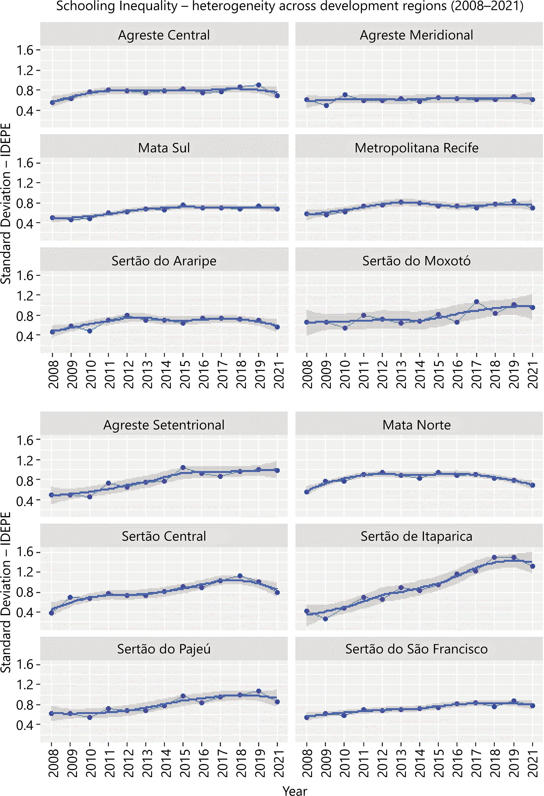
After this, we explored the trajectory of Schooling Effectiveness and Schooling Inequality within each development region across the years. Figure 3 shows multi panels with the mean of Idepe, and Figure 4 the standard deviation of the Idepe, both for each of the 12 development regions and respective trend lines, from 2008-2021.
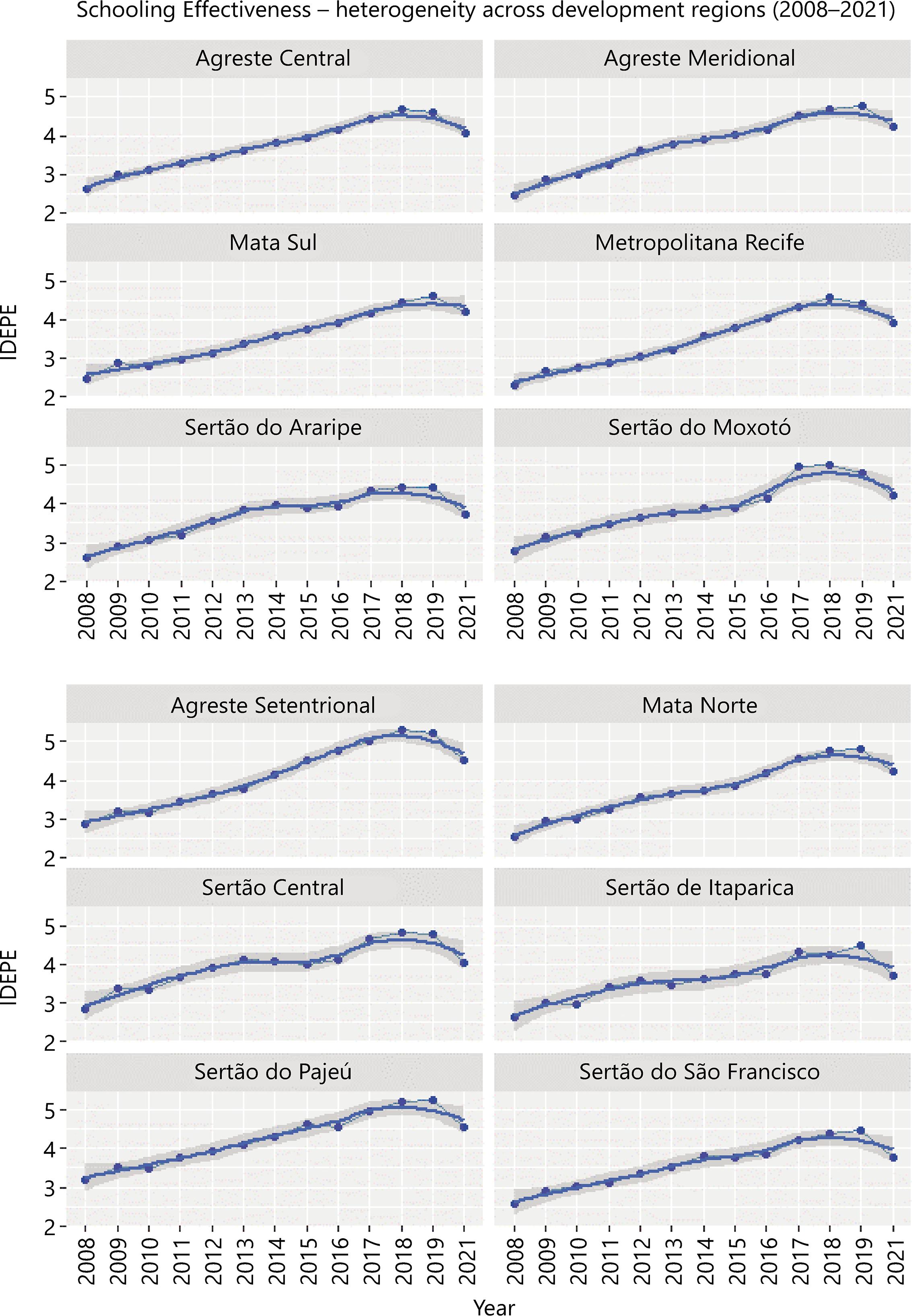
Source: Own elaboration (2024)
Figure 3 Multi panels with the mean of Idepe for Pernambuco’s all 12 development regions from 2008-2021
3.3 Schooling Inequality
The schooling inequality analysis in this paper follows Ram’s (1990) paper, which appropriates the CK in Education. The main idea is that increasing schooling effectiveness may lead to increasing schooling inequality. Theoretically, the relationship is curvilinear; with the increase in effectiveness, the inequity would grow until it reaches a maximum point, from where it would reduce.
Since the Idepe is the used metric for Education effectiveness, we used the standard deviation of the Idepe as a proxy for schooling inequality, and the idepe and its quadratic term to test the linear and/or quadratic relation (positive or negative) between increasing effectiveness and expanding schooling inequality (Ram, 1990; Neves; Almeida, 2016).
As control variables, we used:
A set of regional development: (1) GDP per capita, (2) schools with internet per capita, and (3) urban schools per capita;
a set of extended journey types to control for school effectiveness: (4) schools with a five days full-time journey per capita, (5) schools with a part-time journey per capita, (6) schools with three days full-time journey per capita, (7) full-time technical schools per capita;
a set of schools’ classes specifications to control for the complexity of Education: (8) schools with night classes per capita, (9) schools with classes for adults per capita;
a set of student social characteristics considering enrollment share to control students’ profile: (10) share of whites, (11) share of women, and (12) share of age-grade distortion for 126h-grade students.
Considering the development region (rd) as the space statistic unit and the year of the test as the time unit, we arrived at the equation below:
With the given equation, we build four model methods: (i) pooled, (ii) first differences - FD, (iii) fixed effects - FE, and (iv) random effects - RE, using R, RStudio, and the plm package (Croissant; Millo, 2008). We displayed the complete models in the appendix.
After model estimation, we performed the Croissant and Millo (2008) and Mesquita, Fernandes and Figueiredo Filho (2021) sequence of tests to decide what model was adequate – as show in Table 1 below:
Table 1 Hypothesis Test for Panel Data Model Selection
| Method | Statistics | P-value | Alternative |
|---|---|---|---|
| F Test | 6.763841 | 0.0000000 | significant effects |
| Breusch-Pagan | 13.098660 | 0.0014311 | significant effects |
| Hausman Test | 123.885897 | 0.0000000 | one model is inconsistent |
| Wooldridge’s first-difference test | 12.580157 | 0.0005429 | serial correlation in differenced errors |
Source: Own elaboration (2024)
F-test for Pooled vs. Fixed Effects. Alternative: significant effects (Fixed Effects are adequate);
Breusch-Pagan Test for Pooled vs. Random Effects. Alternative: significant effects (Random Effects is adequate);
Hausman Test for Random Effects vs. Fixed Effects: Alternative: one model is consistent (Fixed Effects estimators will be consistent);
Wooldridge first–difference–based Test for First-Difference vs. Fixed Effects. Alternative: serial correlation in differenced errors (Fixed Effects are adequate since we put First-Difference asNull hypothesis).
Upon identifying that Fixed Effects were adequate, we performed two procedures: i) reorganize variables searching for best fit; ii) follow up analysis to see if the model residuals were normal and if there was a serial correlation or cross-sectional dependence.
Specifically, we present the final model with Idepe, Idepe2, Part-time Schools, Technical Full-time Schools, Urban Schools, and Scholls with Internet variables. We performed the Shapiro-Wilk normality test, Wooldridge’s test for serial correlation in FE, and the Pesaran CD test for panel cross-sectional dependence – as show in Table 2 below.
Table 2 Hypothesis Test for Panel Data Model Assumption
| Method | Statistics | p_value | Alternative | |
|---|---|---|---|---|
| W | Shapiro-Wilk | 0.995983 | 0.9506671 | Non-normally distributed |
| F | Wooldridge’s Test | 3.106286 | 0.0801421 | serial correlation |
| Z | Pesaran CD Test | -2.520897 | 0.0117056 | cross-sectional dependence |
Source: Own elaboration (2024)
The residuals have a normal distribution and no serial correlation, but there is cross-sectional dependence, which demands robust estimators, like Beck and Katz’s (1995) Panel Corrected Standard Errors (PCSE). The Table 3 shows the final model with original and robust estimators.
Table 3 Original and Robust Estimators
| Schooling Inequality - Fixed Effects | ||
|---|---|---|
| Dependent variable: | ||
| Standard Deviation – IDEPE | ||
| Panel linear | Coefficient Test | |
| Fixed Effects | PCSE | |
| (1) | (2) | |
| Idepe | -0.658*** | -0.658*** |
| (0.199) | (0.235) | |
| Idepe2 | 0.094*** | 0.094*** |
| (0.024) | (0.027) | |
| Part-time Schools | 0.020** | 0.020** |
| (0.009) | (0.009) | |
| Technical Full-time Schools | 0.121** | 0.121* |
| (0.057) | (0.070) | |
| Urban Schools | -0.060*** | -0.060*** |
| (0.015) | (0.019) | |
| Continue | ||
| Schools with Internet | 0.061*** | 0.061*** |
| (0.008) | (0.008) | |
| Observations | 156 | |
| R2 | 0.587 | |
| Adjusted R2 | 0.492 | |
| F Statistic | 29.891*** (df = 6; 126) | |
Source: Own elaboration (2024)
*p < 0.1; **p < 0.05; ***p < 0.01
4 Discussion
As seen in Figure 1, Schooling Effectiveness has increased over the years. Also, as shown in Figure 2, Schooling Inequality has increased over the years in the overall mean of development regions. It indicates that advances in effectiveness are generally followed closely by advances in inequality.
However, Figures 3 and 4 indicate that (i) both effectiveness and inequality have substantial variation among different development regions and (ii) although effectiveness has an everlasting ascendent trend for all regions, inequality follows different patterns across the regions and the years.
The panel data model was robust to the hypothesis test applied and showed an excellent capacity to explain the variability (with Adjusted R2 of 0.492), being practical in helping to understand better the effects of different aspects of effectiveness over inequality.
Considering the effectiveness vs. inequality relation, the positive coefficient of the quadratic term of Idepe and the negative coefficient of Idepe indicate that the relationship follows a regular-U shape, in which, as effectiveness grows, inequality decreases until a minimum point from where it starts to increase.
Regarding typology, development, and localization, it is noticeable that the inequality is higher in regions where we find more part-time schools without extended journeys, regions with more technical full-time schools, and regions with more schools with internet. On the other hand, regions with more urban schools tend to have lower inequality. It is then necessary to examine the trajectory of these variables across time.
Figure 5 shows that typology varies across time, with the total of part-time schools (no extended journey) decreasing over the years, while the total of full-time technical schools has increased during the same period.
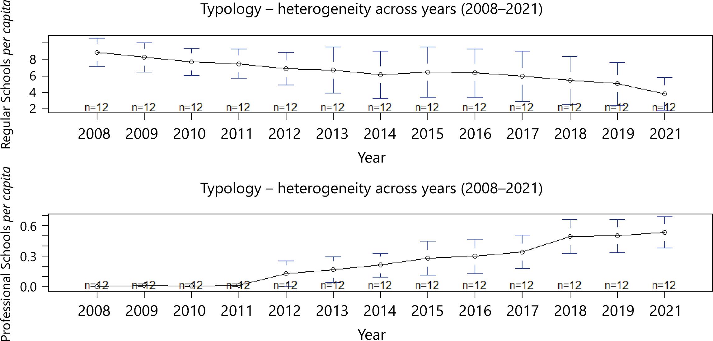
Source: Own elaboration (2024)
Figure 5 Number of part-time and technical full-time schools in Pernambuco’s all 12 development regions from 2008-202110
On the other hand, Figure 6 shows that the schools with internet and the urban schools are very stable over time. The first showed an increase and stabilized, while the second oscillated around a central value since the beginning of the period.
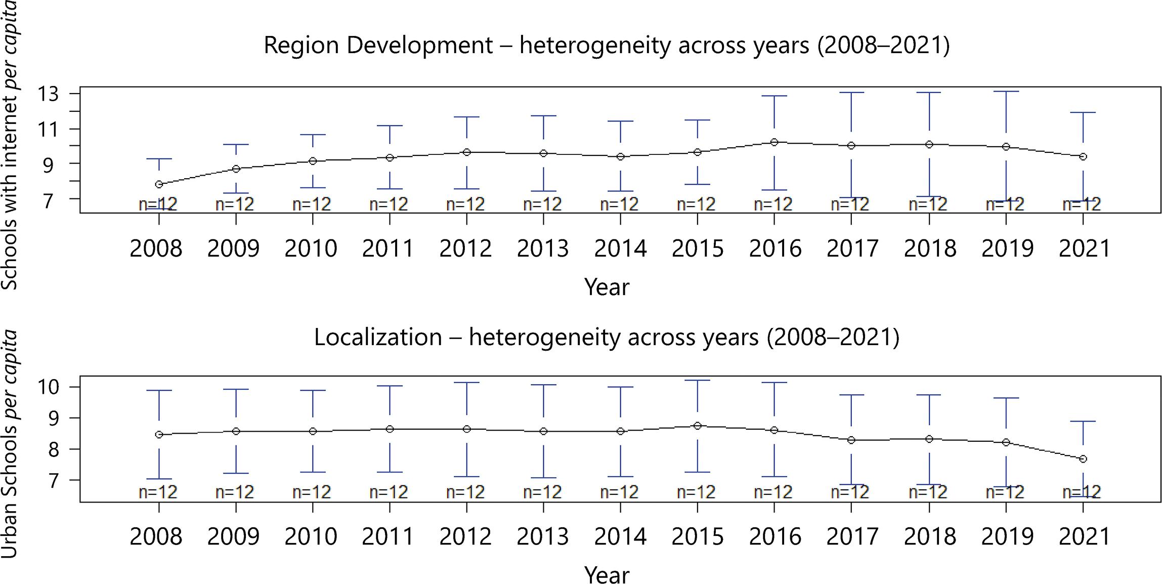
Source: Own elaboration (2024)
Figure 6 Number of urban schools and schools with no internet access in Pernambuco’s all 12 development regions from 2008-2021
In sum, we can say that (i) effectiveness and inequality are growing across time, (ii) the relation between the two aspects follows a regular-U shape, (iii) some typology variables are changing across time that affects inequality positively, (iv) some other aspects are more stable across time but may vary across regions, which also affects inequality, (v) in general, regions with more extended journey schools tend to show smaller schooling inequality.
5 Conclusion
Considering the previous studies on full-time Education in Brazil, as Neves and Almeida (2016), we identified that Kuznets-hypothesis on Education is also present in using standardized test scores as effectiveness, noticing that this type of Education is not salvationist (Castanho; Mancini, 2016; Silva; Jófili, 2022), as it comes with its contradictions and externalities
It is possible to infer that the equity of the result is more connected to the effects of the diversity of school typology (quite variable over the years), the location of schools (fixed over time), and the way that a region is developed (which also may be constant over time). These findings are comparable to Blanco and Ram (2019), in which the relationship has a regular-U shape.
In the case of Pernambuco and its trajectory of increase in the number of extended journey schools, development regions with more urban schools and a more homogeneous school typology of extended journey schools tend to present better equity of results. Equity that, for the case in question, is also influenced by the achievement of the result itself, i.e., by the effectiveness of the Education. So, policymakers should put effort to create policies that address not only socioeconomic inequalities, but also schoolling inequalities, since the expected course of developing policies seems to be to increase even more the results of better units.
One possible limitation of this study relates to the assumption that the standardized test remained the same - or at least with minimum conditions - across all years of analysis. That is, since IRT has robust premises that are not directly verified with the available data, we assumed that all years on the dataset followed the expected IRT conditions. However, gaming is always possible, i.e., some schools may be “playing with the rules” to produce the best results possible (Hood, 2007; Segatto; Abrucio, 2017). Nevertheless, in both cases, the autoEDA (especially the missing at-random analysis) and the panel data models do not indicate relevant problems, leading to the belief that variations due to changes in specification tests or gaming are stochastic.
Another limitation of the studies that apply Kuznets-hypothesis to Education is related to the measure of inequality and the use of controls. As Shukla and Mishra (2019) identified, the relationship between effectiveness and inequality may change signals depending on the measure used. Also, the association between inequality and social, economic, and typology aspects may change due to study design choices and the disponibility of the data11.
To better address these questions, future studies would include controls about teachers and families while retaining other controls used here, especially typology, because of the relationship between extended journey and effectiveness (Araújo et al., 2020; Battistin; Meroni, 2016; Fukushima; Quintão; Pazello, 2022; Huebner; Kuger; Marcus, 2017; Rosa et al., 2020; Schüpbach, 2014). Another possibility is to use data on the student level, aggregated by class or even school - which is currently unavailable due to personal data protection. It would also be ideal for observing the relation between effectiveness and equality using other measures since each one captures different publics of Education: years of educational attainment measures general Education, but standardized tests, as Idepe, measure the 12th-grade covering only mathematics and language. Finally, it would be interesting to model using different measures of dispersion (standard deviation, Gini index, et cetera).

